Unidirectional imaging using deep learning–designed materials
JINGXI LI, TIANYI GAN, YIFAN ZHAO, BIJIE BAI, , CHE-YUNG SHEN, SONGYU SUN, MONA JARRAHI AND AYDOGAN OZCAN
A unidirectional imager would only permit image formation along one direction, from an input field-of-view (FOV) A to an output FOV B, and in the reverse path, B → A, the image formation would be blocked. We report the first demonstration of unidirectional imagers, presenting polarization-insensitive and broadband unidirectional imaging based on successive diffractive layers that are linear and isotropic. After their deep learning–based training, the resulting diffractive layers are fabricated to form a unidirectional imager. Although trained using monochromatic illumination, the diffractive unidirectional imager maintains its functionality over a large spectral band and works under broadband illumination. We experimentally validated this unidirectional imager using terahertz radiation, well matching our numerical results. We also created a wavelength-selective unidirectional imager, where two unidirectional imaging operations, in reverse directions, are multiplexed through different illumination wavelengths. Diffractive unidirectional imaging using structured materials will have numerous applications in, e.g., security, defense, telecommunications, and privacy protection.
We kindly thank the researchers at University of California for this collaboration, and for sharing the results obtained with their system.

Introduction
Optical imaging applications have permeated every corner of modern industry and daily life. A myriad of optical imaging methods have flourished along with the progress of physics and information technologies, resulting in imaging systems such as super-resolution microscopes (1, 2), space telescopes (3–5), and ultrafast cameras (6, 7) that cover various spatial and temporal scales at different bands of the electromagnetic spectrum. With the recent rise of machine learning technologies, researchers have also started using deep learning algorithms to design optical imaging devices based on massive image data and graphics processing units, achieving optical imaging designs that, in some cases, surpass what can be obtained through physical intuition and engineering experience (8–14).
Standard optical imaging systems composed of linear and time-invariant components are reciprocal, and the image formation process is maintained after swapping the positions of the input and output fields of view (FOVs). If one could introduce a unidirectional imager, then the imaging black box would project an image of an input object FOV (A) onto an output FOV (B) through the forward path (A → B), whereas the backward path (B → A) would inhibit the image formation process by scattering the optical fields outside the output FOV (see Fig. 1A).
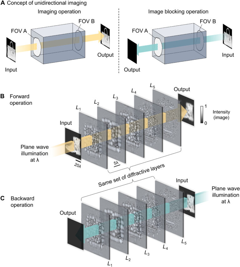
Fig. 1. Schematic of a diffractive unidirectional imager. (A) Concept of unidirectional imaging, where the imaging operation can be performed as the light passes along a certain specified direction (A → B), while the image formation is blocked along the opposite direction (B → A). (B and C) Illustration of our diffractive unidirectional imager, which performs imaging of the input FOV with high fidelity in its forward (B) direction and blocks the image formation in its backward (C) direction. This diffractive unidirectional imager is a reciprocal device that is linear and time invariant and provides asymmetric optical mode processing in the forward and backward directions. Its design is insensitive to light polarization and leaves the input polarization state unchanged at its output. Furthermore, it maintains its unidirectional imaging functionality over a large spectral band and works under broadband illumination.
To design a unidirectional imager, one general approach would be to break electromagnetic reciprocity: One can use, e.g., magneto-optic effect (the Faraday effect) (15–17), temporal modulation of the electromagnetic medium (18, 19), or other nonlinear optical effects (20–27). However, realizing such nonreciprocal systems for unidirectional imaging over a sample FOV with many pixels poses challenges due to high fabrication costs, bulky and complicated setups/materials, and/or high-power illumination light sources. Alternative approaches have also been used to achieve unidirectional optical transmission from one point to another without using optical isolators. One of the most common practices is using a quarter-wave plate and a polarization beam splitter; this approach for point-to-point transmission is polarization sensitive and results in an output with only circular polarization. Other approaches include using asymmetric isotropic dielectric gratings (28–31) and double-layered metamaterials (32) to create different spatial mode transmission properties along the two directions. However, these methods are designed for relatively simple input modes and face challenges in off-axis directions, thus making them difficult to form imaging systems even with relatively low numerical apertures.
Despite all the advances in materials science and engineering and optical system design, there is no unidirectional imaging system reported to date, where the forward imaging process (A → B) is permitted and the reverse imaging path (B → A) is all optically blocked.
Here, we report the first demonstration of unidirectional imagers and design polarization-insensitive and broadband unidirectional imaging systems based on isotropic structured linear materials (see Fig. 1, B and C). Without using any lenses commonly used in imaging, here, we optimize a set of successive dielectric diffractive layers consisting of hundreds of thousands of diffractive features with learnable thickness (phase) values that collectively modulate the incoming optical fields from an input FOV. After being trained using deep learning (33–46), the resulting diffractive layers are physically fabricated to form a unidirectional imager, which performs polarization-insensitive imaging of the input FOV with high structural fidelity and power efficiency in the forward direction (A → B), while blocking the image transmission in the backward direction, not only penalizing the diffraction efficiency from B → A but also losing the structural similarity or resemblance to the input images. Despite being trained using only Modified National Institute of Standards and Technology (MNIST) handwritten digits, these diffractive unidirectional imagers are able to generalize to more complicated input images from other datasets, demonstrating their external generalization capability and serving as a general-purpose unidirectional imager from A → B. Although these diffractive unidirectional imagers were trained using monochromatic illumination at a wavelength of λ, they maintain unidirectional imaging functionality under broadband illumination, over a large spectral band that uniformly covers, e.g., 0.85 × λ to 1.15 × λ.
We experimentally confirmed the success of this unidirectional imaging concept using terahertz waves and a three-dimensional (3D) printed diffractive imager and revealed a very good agreement with our numerical results by providing clear and intense images of the input objects in the forward direction and blocking the image formation process in the backward direction. Using the same deep learning–based training strategy, we also designed a wavelength-selective unidirectional imager that performs unidirectional imaging along one direction (A → B) at a predetermined wavelength and along the opposite direction (B → A) at another predetermined wavelength. With this wavelength-multiplexed unidirectional imaging design, the operation direction of the diffractive unidirectional imager can be switched (back and forth) based on the illumination wavelength, improving the versatility and flexibility of the imaging system.
The optical designs of these diffractive unidirectional imagers have a compact size, axially spanning ~80 to 100λ. Such a thin footprint would allow these unidirectional imagers to be integrated into existing optical systems that operate at various scales and wavelengths. While we considered here spatially coherent illumination, the same design framework and diffractive feature optimization method can also be applied to spatially incoherent scenes. Polarization-insensitive and broadband unidirectional imaging using linear and isotropic structured materials will find various applications in security, defense, privacy protection, and telecommunications among others.
Results
Diffractive unidirectional imager using reciprocal structured materials
Figure 1A depicts the general concept of unidirectional imaging. To create a unidirectional imager using reciprocal structured materials that are linear and isotropic, we optimized the structure of phase-only diffractive layers (i.e., L1, L2, …, L5), as illustrated in Fig. 1 (B and C). In our design, all the diffractive layers share the same number of diffractive phase features (200 by 200), where each dielectric feature has a lateral size of ~λ/2 and a trainable/learnable thickness providing a phase modulation range of 0 to 2π. The diffractive layers are connected to each other and the input/output FOVs through free space (air), resulting in a compact system with a total length of 80λ (see Fig. 2A). The thickness profiles of these diffractive layers were iteratively updated in a data-driven fashion using 55,000 distinct images of the MNIST handwritten digits (see Materials and Methods). A custom loss function is used to simultaneously achieve the following three objectives: (i) minimize the structural differences between the forward output images (A → B) and the ground truth images based on the normalized mean square error (MSE), (ii) maximize the output diffraction efficiency (overall transmission) in the forward path, A → B, and (iii) minimize the output diffraction efficiency in the backward path, B → A. More information about the architecture of the diffractive unidirectional imager, loss functions, and other training-related implementation details can be found in Materials and Methods. After the completion of the training, the phase modulation coefficients of the resulting diffractive layers are shown in Fig. 2C. Upon closer inspection, it can be found that the phase patterns of these diffractive layers have stronger modulation in their central regions, while the edge regions appear relatively smooth, with weaker phase modulation. This behavior can be attributed to the size difference between the smaller input/output FOVs and the relatively larger diffractive layers, which causes the edge regions of the diffractive layers to receive weaker waves from the input, as a result of which their optimization remains suboptimal.
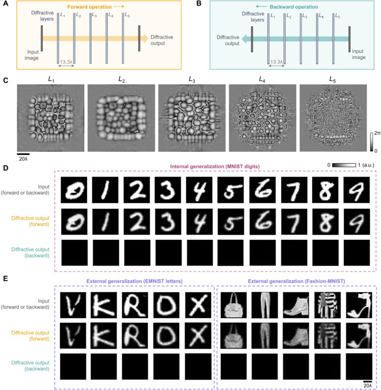
Fig. 2. Design schematic and blind testing results of the diffractive unidirectional imager. (A and B) Layout of the diffractive unidirectional imager when it operates in the forward (A) and backward (B) directions. (C) The resulting diffractive layers of a diffractive unidirectional imager. (D) Exemplary blind testing input images taken from Modified National Institute of Standards and Technology (MNIST) handwritten digits that were never seen by the diffractive imager model during its training, along with their corresponding diffractive output images in the forward and backward directions. a.u., arbitrary units. (E) Same as (D), except that the testing images are taken from the Extended MNIST (EMNIST) and Fashion-MNIST datasets, demonstrating external generalization to more complicated image datasets.
This diffractive unidirectional imager design was numerically tested using the MNIST test dataset, which consists of 10,000 handwritten digit images that were never seen by the diffractive model during the training process. We report some of these blind testing results in Fig. 2D for both the forward and backward directions, clearly illustrating the internal generalization of the resulting diffractive imager to previously unseen input images from the same dataset. We also quantified the performance of this diffractive unidirectional imager for both the forward and backward directions based on the following metrics: (i) the normalized MSE and (ii) the Pearson correlation coefficients (PCCs) between the input and output images (denoted as “output MSE” and “output PCC”) and (iii) the output diffraction efficiencies; these metrics were calculated using the same set of MNIST test images, never seen before. As shown in Fig. 3 (A and B), the forward (A → B) and backward (B → A) paths of the diffractive unidirectional imager shown in Fig. 2C provide output MSE values of (5.68 ± 1.56) × 10−5 and (0.919 ± 0.048) × 10−3, respectively, and their output PCC values are calculated as 0.9740 ± 0.0065 and 0.3839 ± 0.0685, respectively. A similar asymmetric behavior between the forward and backward imaging directions is also observed for the output diffraction efficiency metric as shown in Fig. 3C: The output diffraction efficiency of A → B is found as 93.50 ± 1.56%, whereas it is reduced to 1.57 ± 0.44% for B → A, which constitutes an average image power suppression ratio of ~60-fold in the reverse direction compared to the forward imaging direction. Equally important as this poor diffraction efficiency for B → A is the fact that the weak optical field in the reverse direction does not have spatial resemblance to the input objects as revealed by a poor average PCC value of ~0.38 for B → A. These results demonstrate and quantify the internal generalization success of our diffractive unidirectional imager: The input images can be successfully imaged with high structural fidelity and power efficiency along the forward direction of the diffractive imager, while the backward imaging operation B → A is inhibited by substantially reducing the output diffraction efficiency and distorting the structural resemblance between the input and output images.
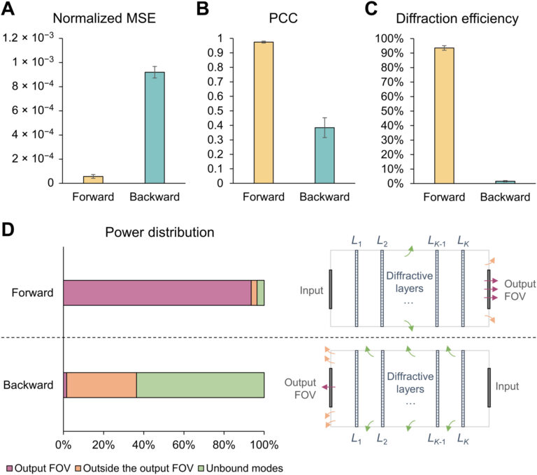
Fig. 3. Performance analysis of the diffractive unidirectional imager shown in Fig. 2. (Aand B) Normalized mean square error (MSE) (A) and Pearson correlation coefficient (PCC) (B) values calculated between the input images and their corresponding diffractive outputs in the forward and backward directions. (C) The output diffraction efficiencies of the diffractive unidirectional imager calculated in the forward and backward directions. In (A) to (C), the metrics are benchmarked across the entire MNIST test dataset and reported here with their mean values and SDs added as error bars. (D) Left: The power of the different spatial modes propagating in the diffractive volume during the forward and backward operations, shown as percentages of the total input power. Right: Schematic of the different spatial modes propagating in the diffractive volume. FOV, field of view.
To better understand the working principles of this diffractive unidirectional imager, next, we consider the 3D space formed by all the diffractive layers and the input/output planes as a diffractive volume and categorize/group the optical fields propagating within this volume as part of different spatial modes: (i) the optical modes that lastly arrive at the target output FOV, i.e., at FOV B for A → B and at FOV A for B → A; (ii) the optical modes arriving at the output plane but outside the target output FOV; and (iii) the unbounded optical modes that do not reach the output planes; since the diffractive layers are axially separated by >10λ, there are no evanescent waves being considered here. We calculated the power distribution percentages of each one of these types of optical modes for both A → B and B → A for each test image and reported their average values across the 10,000 test images in Fig. 3D (see Materials and Methods for details). The results summarized in Fig. 3D clearly reveal that, in the forward path (A → B) of the diffractive unidirectional imager, the majority of the input power (>93.5%) is coupled to the imaging modes that arrive at the output FOV B, forming high-quality images of the input objects with a mean PCC of 0.974, while the optical modes that fall outside the FOV B and the unbound modes are minimal, accounting for only ~2.95 and ~3.54% of the input total power, respectively. In contrast, the backward imaging path (B → A) of the same diffractive unidirectional imager steers most of the input power into the nonimaging modes that fall outside the FOV A or escape out of the diffractive volume through the unbounded modes, which correspond to power percentages of ~34.8 and ~63.6%, respectively. For B → A, the optical modes that arrive at the FOV A only constitute, on average, ~1.57% of the input total power; however, these optical modes are not only weak but also substantially aberrated by the diffractive unidirectional imager, resulting in very poor output images, with a mean PCC value of ~0.38.
The underlying reason for these contrasting power distributions in the two imaging directions stems from the different order of the diffractive layers as the light passes through them. This can be further confirmed through the analyses reported in fig. S1, where we provided a visualization of the variation of the optical fields propagating within the same diffractive design. As shown in fig. S1C, in the forward operation, A → B, the diffractive layers arranged in the order of L1 to L5 manage to maintain most of the light waves at the central regions throughout the wave propagation such that the input image is efficiently focused within output FOV B to form high-quality output images. In contrast, in the backward operation, B → A, as shown in fig. S1D, the same set of diffractive layers arranged in the reversed order (i.e., L5 to L1) scatter the transmitted input optical fields and couple them into nonimaging modes (i.e., unbound modes that leave the diffractive imager volume and modes that end up outside the output image FOV); both of these set of modes never arrive at the output image FOV A. In addition to this, for the backward operation, B → A, the diffractive layers ordered in the reverse direction (L5 to L1) scramble the distributions of the optical fields that arrive at FOV A, suppressing their structural resemblance to the input images.
Note that, since the presented diffractive unidirectional imager is composed of linear, time-invariant and isotropic materials, it forms a reciprocal system that is polarization insensitive. In experimental implementations (reported below) due to absorption-related losses, a diffractive unidirectional imager also exhibits time-reversal asymmetry.
To further highlight the capabilities of our diffractive unidirectional imager (which was trained using handwritten digits), we also tested its external generalization using other datasets: The Extended MNIST (EMNIST) dataset that contains images of handwritten English letters and the Fashion-MNIST dataset that contains images of various fashion products. The blind testing results on these two additional datasets using the diffractive unidirectional imager of Fig. 2C are exemplified in Fig. 2E, which once again confirm its success. As another demonstration of the external generalization of our diffractive unidirectional imager, we reversed the contrast of the images in these test datasets, where the light transmitting and blocking regions of the input images were swapped, further deviating from our training image set. The results of this analysis are presented in fig. S2, demonstrating successful unidirectional imaging using our diffractive design, irrespective of the test image dataset and the contrast of the input image features.
In addition to these, we quantified the imaging resolution performance of this diffractive unidirectional imager using gratings as resolution test targets, which were also never used in the training phase (see Fig. 4). Our results reveal that the diffractive unidirectional imager can resolve a minimum linewidth of ~4λ in the forward path, A → B, while successfully inhibiting the image formation in the reverse path, B → A, as expected. These results once again prove that the training of the diffractive unidirectional imager is successful in approximating a general-purpose imaging operation in the forward path, although we only used handwritten digits during its training.
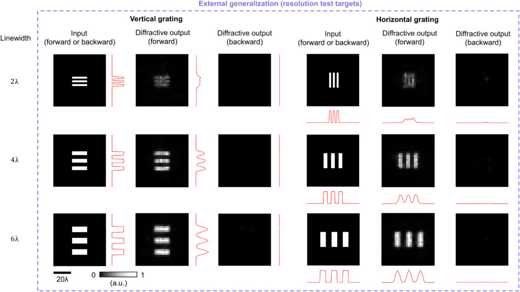
Fig. 4. Spatial resolution analysis for the diffractive unidirectional imager shown in Fig. 2. Resolution test target images composed of grating patterns with different periods and orientations and their corresponding diffractive output images are shown for both the forward and backward imaging directions. The red lines indicate the one-dimensional (1D) cross-sectional profiles calculated by integrating the intensity of the grating patterns in the diffractive output images along the direction perpendicular to the grating.
Spectral response of the diffractive unidirectional imager
Next, we explored the spectral response of the diffractive unidirectional imager reported in Fig. 2 under different illumination wavelengths that deviate from the training illumination wavelength (λtrain = λ). The results of this analysis are reported in Fig. 5 (A and B), where the output image PCC and diffraction efficiency values of the diffractive unidirectional imager of Fig. 2 were tested as a function of the illumination wavelength. Although this diffractive unidirectional imager was only trained at a single illumination wavelength (λ), it also works well over a large spectral range as shown in Fig. 5 (A and B). Our results reveal that the imaging performance in the forward path (A → B) remains very good with an output image PCC value of ≥0.85 and an output diffraction efficiency of ≥85.5% within the entire spectral range [λL : λR], where λL = 0.92 × λ and λR = 1.11 × λ (see Fig. 5, A and B). Within the same spectral range defined by [λL : λR], the power suppression ratio between the forward and backward imaging paths always remains ≥17.4×, and the output diffraction efficiency of the reverse path (B → A) remains ≤5.49% (see Fig. 5B), indicating the success of the diffractive unidirectional imager over a large spectral band, despite the fact that it was only trained with monochromatic illumination at λ. Figure 5D further reports examples of test objects (never seen during the training) that are simultaneously illuminated by a continuum of wavelengths, covering two different broadband illumination cases: (i) [0.92 × λ : 1.11 × λ] and (ii) [0.85 × λ : 1.15 × λ]. The forward and backward imaging results for these two broadband illumination cases shown in Fig. 5D clearly illustrate the success of the diffractive unidirectional imager under broadband illumination.
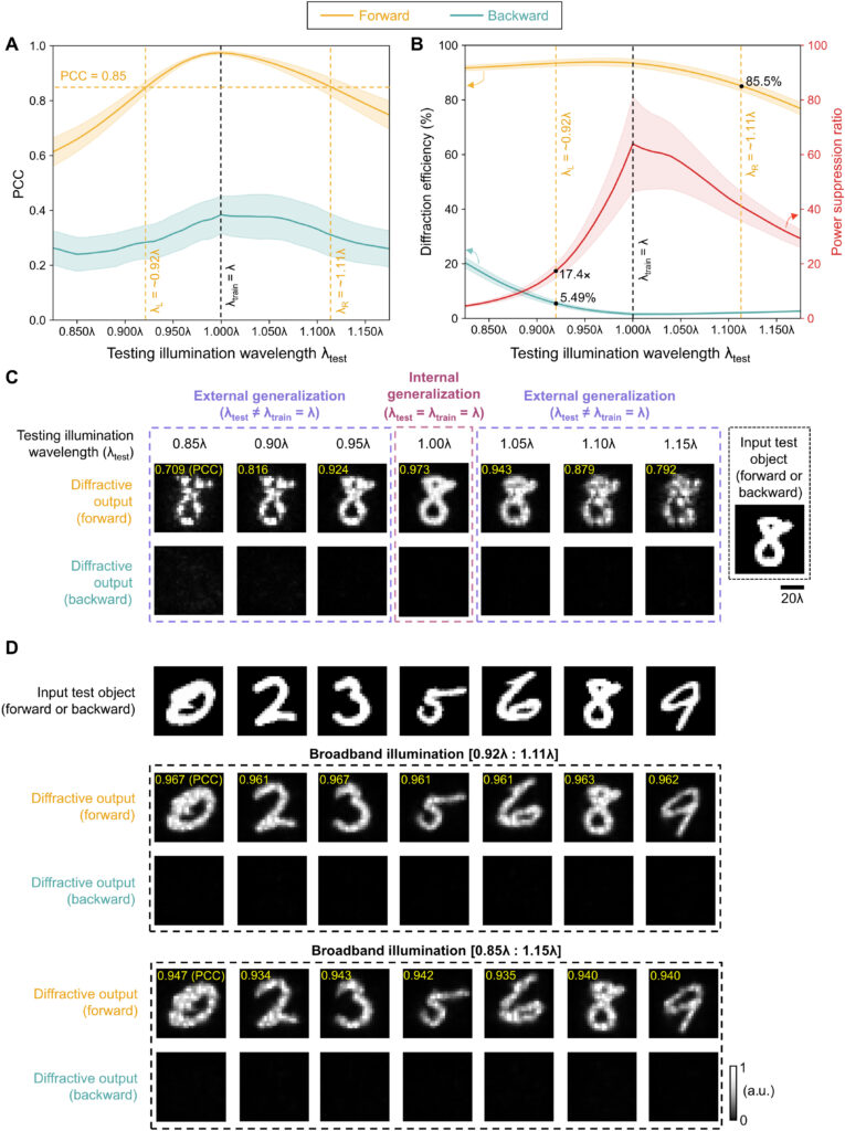
Fig. 5. Spectral response of the diffractive unidirectional imager design shown in Fig. 2. (A and B) Output image PCC (A) and diffraction efficiency (B) of the diffractive unidirectional imager in the forward and backward directions as a function of the illumination wavelength used during the blind testing. The values of the power suppression ratio are also reported in (B), which refers to the ratio between the output diffraction efficiency of the forward operation and the backward operation. The shaded areas indicate the SD values calculated based on all the 10,000 images in the testing dataset. (C) Examples of the output images in the forward and backward directions when using different illumination wavelengths during the testing, along with the corresponding input test images (never used during the training). (D) Broadband illumination results for several test objects are shown for the forward and backward imaging directions. Two different broadband illumination cases are shown, uniformly covering (i) 0.92 × λ to 1.11 × λ and (ii) 0.85 × λ to 1.15 × λ, where λ is the training illumination wavelength, λtrain = λ.
We should emphasize that these broadband unidirectional imaging results can be further enhanced by training the diffractive layers using a set of wavelengths sampled from a desired spectral band, as an alternative to using a single training wavelength. The validity of this approach is confirmed by an additional analysis reported in fig. S7 (A and B), which compares the spectral response of the model shown in Fig. 2 to that of another diffractive model trained using the same configuration and hyperparameters, but with the operational wavelength selected randomly within the spectral range of [λL : λR] during the training process, where λL = 0.92 × λ and λR = 1.11 × λ. As shown in fig. S7C, this training approach with a wide continuum of wavelengths substantially improves the output PCC values in the forward direction at illumination wavelengths far away from the center wavelength λ. These advantages of the broadband design also come at the expense of relatively reduced peak PCC values of the forward output images at λ and a small reduction in the forward diffraction efficiency.
Experimental validation of the diffractive unidirectional imager design
We experimentally validated our diffractive unidirectional imager using a monochromatic continuous-wave terahertz illumination at λ = 0.75 mm, as shown in Fig. 6A. A schematic diagram of the terahertz setup is shown in Fig. 6B, and its implementation details are reported in Materials and Methods. For this experimental validation, we designed a diffractive unidirectional imager composed of three diffractive layers, where each layer contains 100 by 100 learnable diffractive features, each with a lateral size of 0.64λ (dictated by the resolution of our 3D printer). The axial spacing between any two adjacent layers (including the diffractive layers and the input/output planes) is chosen as ~26.7λ. Different from earlier designs, here, we also took into account the material absorption using the complex-valued refractive index of the diffractive material in our optical model, such that the optical fields absorbed by the diffractive layers are also considered in our design (which will be referred to as the “absorbed modes” in the following discussion). Moreover, to overcome the undesired performance degradation that may be caused by the misalignment errors in an imperfect physical assembly of the diffractive layers, we also adopted a “vaccination” strategy in our design by introducing random displacements applied to the diffractive layers during the training process, which enabled the final converged diffractive unidirectional imager to become more resilient to potential misalignment errors (see Materials and Methods).
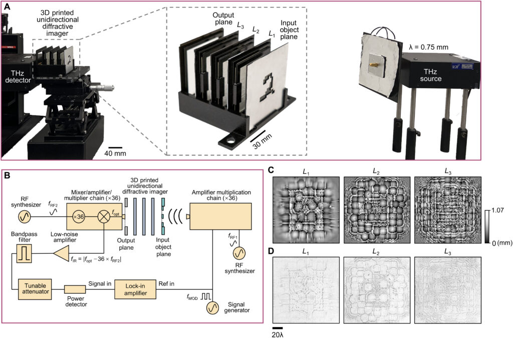
After the training was complete, we conducted numerical performance analysis for this converged diffractive design using blind testing objects, with the results shown in fig. S3. Upon comparison to the earlier model presented in Fig. 2, which had a high output diffraction efficiency of >90% in its forward direction, we found that this experimental design exhibits a relatively lower diffraction efficiency of ~21.33% in the forward imaging direction, A → B. This power efficiency reduction can be attributed to two main factors: (i) The existence of absorption by the diffractive layers caused ~27% of the input power to be lost through the absorbed modes; and (ii) our experimental design choice of using fewer diffractive layers (i.e., three layers) resulted in a reduced number of trainable diffractive features, leading to a larger portion of the input power (~46%) converted to the unbound modes. Nevertheless, this experimental design still maintains a substantially higher forward diffraction efficiency when compared to the backward direction, where ~1.8% of the input energy enters the output FOV (FOV A) in the reverse direction, B → A. Moreover, the forward and backward PCC values for this experimental design stand at 0.9618 ± 0.0100 and 0.4859 ± 0.0710, respectively, indicating the success of the unidirectional imager design.
After the training, the resulting diffractive layers were fabricated using a 3D printer (Fig. 6, C and D). In our experiments, we tested the performance of this 3D fabricated diffractive unidirectional imager along the forward and backward directions, as illustrated in Fig. 7 (A and B). Ten different handwritten digit samples from the blind testing set (never used in the training) were used as the input test objects, also 3D printed. These experimental imaging results for A → B and B → A are shown in Fig. 7C, which present a good agreement with their numerical simulated counterparts, very well matching the input images. As expected, 3D printed diffractive unidirectional imager faithfully imaged the input objects in its forward direction and successfully blocked the image formation in the backward direction; these results constitute the first demonstration of unidirectional imaging.
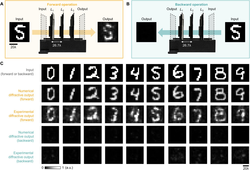
Fig. 7. Experimental results. (A and B) Layout of the diffractive unidirectional imager that was fabricated for experimental validation when it operates in the forward (A) and backward (B) directions. (C) Experimental results of the unidirectional imager using the fabricated diffractive layers.
Wavelength-multiplexed unidirectional diffractive imagers
Next, we consider a more challenging task: combining two diffractive unidirectional imagers that operate in opposite directions, where the direction of imaging is controlled by the illumination wavelength. The resulting diffractive system forms a wavelength-multiplexed unidirectional imager, where the image formation from A → B and B → A is maintained at λ1 and λ2 illumination wavelengths, respectively, whereas the image formation from B → A and A → B is blocked at λ1 and λ2, respectively (see Figs. 8 and 9). To implement this wavelength-multiplexed unidirectional imaging concept, we designed another diffractive imager that operates at λ1 and λ2 = 1.13 × λ1 wavelengths and used an additional penalty term in the training loss function to improve the performance of the image blocking operations in each direction, A → B and B → A. More details about the numerical modeling and the training loss function for this wavelength-multiplexed diffractive design can be found in Materials and Methods.
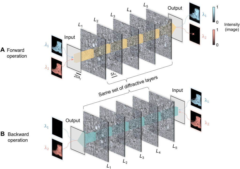
Fig. 8. Illustration of the wavelength-multiplexed unidirectional diffractive imager. In this diffractive design, the image formation operation is performed along the forward direction at wavelength λ1 and the backward direction at λ2, while the image blocking operation is performed along the backward direction at λ1 and the forward direction at λ2. This diffractive imager works as a unidirectional imaging system at two different wavelengths, each with a reverse imaging direction with respect to the other. λ2 = 1.13 × λ1.
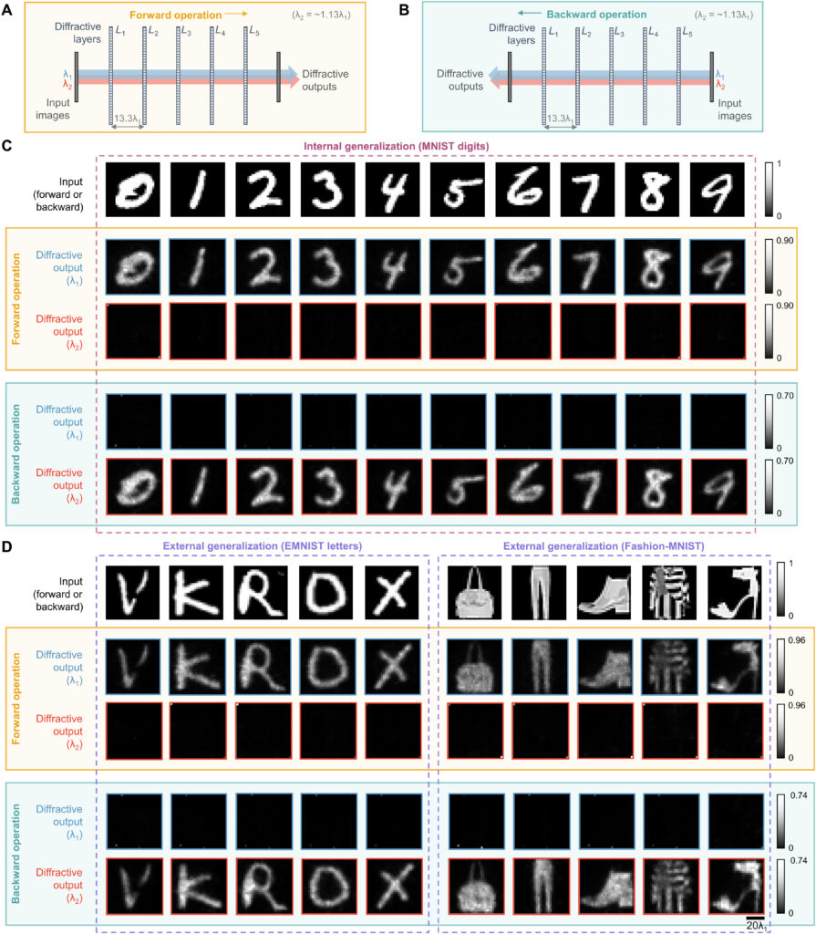
Fig. 9. Design schematic and blind testing results of the wavelength-multiplexed unidirectional diffractive imager. (A and B) Layout of the wavelength-multiplexed unidirectional diffractive imager when it operates in the forward (A) and backward (B) directions. (C) Exemplary blind testing input images taken from MNIST handwritten digits that were never seen by the diffractive imager model during its training, along with their corresponding diffractive output images at different wavelengths in the forward and backward directions. (D) Same as (C) except that the testing images are taken from the EMNIST and Fashion-MNIST datasets, demonstrating external generalization.
We trained this wavelength-multiplexed unidirectional diffractive imager using handwritten digit images as before; the resulting, optimized diffractive layers are reported in fig. S4. Following its training, the diffractive imager was blindly tested using 10,000 MNIST test images that were never used during the training process, with some representative testing results presented in Fig. 9C. These results indicate that the wavelength-multiplexed diffractive unidirectional imager successfully performs two separate unidirectional imaging operations, in reverse directions, the behavior of which is controlled by the illumination wavelength; at λ1, A → B image formation is permitted and B → A is blocked, whereas at λ2, B → A image formation is permitted and A → B is blocked.
We also analyzed the imaging performance of this wavelength-multiplexed unidirectional diffractive imager as shown in Fig. 10 (A to C). At the first wavelength channel λ1, the output PCC values for the forward (A → B) and backward (B → A) directions are calculated as 0.9428 ± 0.0154 and 0.1228 ± 0.0985, respectively, revealing an excellent image quality contrast between the two directions (see Fig. 10B). Similarly, the output diffraction efficiencies for the forward and backward directions at λ1 are quantified as 65.82 ± 3.57 and 3.62 ± 0.72%, respectively (Fig. 10C). In contrast, the second wavelength channel λ2 of this diffractive model performs unidirectional imaging along the direction opposite to that of the first wavelength, providing output PCC values of 0.9378 ± 0.0187 (B → A) and 0.0840 ± 0.0739 (A → B) (see Fig. 10B). Similarly, the output diffraction efficiencies at λ2 were quantified as 51.81 ± 3.77 (B → A) and 2.57 ± 0.36% (A → B). These findings can be further understood by investigating the power distribution within this wavelength-multiplexed unidirectional diffractive imager, which is reported in Fig. 10D. This power distribution analysis within the diffractive volume clearly shows how two different wavelengths (λ1 and λ2) along the same spatial direction (e.g., A → B) can result in very different distributions of spatial modes, performing unidirectional imaging in opposite directions, following the same physical behavior reported in Fig. 3D, except that this time it is wavelength-multiplexed, controlling the direction of imaging. Such an exotic wavelength-multiplexed unidirectional imaging system cannot be achieved using simple spectral filters such as absorption or thin-film filters, since the use of a spectral filter at one wavelength channel (for example, to block A → B at λ2) would immediately also block the reverse direction (B → A at λ2), violating the desired goal.
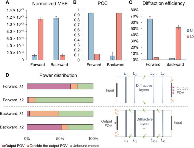
Fig. 10. Performance analysis of the wavelength-multiplexed unidirectional diffractive imager shown in Fig. 9 and fig. S2. (A and B) Normalized MSE (A) and PCC (B) values calculated between the input images and their corresponding diffractive outputs at different wavelengths in the forward and backward operations. (C) The output diffraction efficiencies of the diffractive imager calculated in the forward and backward operations. In (A) to (C), the metrics are benchmarked across the entire MNIST test dataset and shown with their mean values and SDs added as error bars. (D) Left: The power of the different spatial modes at the two wavelengths propagating in the diffractive volume during the forward and backward operations, shown as percentages of the total input power. Right: Schematic of the different spatial modes propagating in the diffractive volume.
We should also note that, since this wavelength-multiplexed unidirectional imager was trained at two distinct wavelengths that control the opposite directions of imaging, the spectral response of the resulting diffractive imager, after its optimization, is vastly different from the broadband response of the earlier designs, reported in, e.g., Fig. 5. Figure S5 reveals that the wavelength-multiplexed unidirectional imager (as desired and expected) switches its spectral behavior in the range between λ1 and λ2, since its training aimed unidirectional imaging at opposite directions at these two predetermined wavelengths. Therefore, this spectral response that is summarized in fig. S5 is in line with the training goals of this wavelength-multiplexed unidirectional imager. However, it still maintains its unidirectional imaging capability over a range of wavelengths in both directions. For example, fig. S5 reveals that the output image PCC values for A → B remain ≥0.85 within the entire spectral range covered by 0.975 × λ1 to 1.022 × λ1 without any considerable increase in the diffraction efficiency for the reverse path, B → A. Similarly, the output image PCC values for B → A remain ≥0.85 within the entire spectral range covered by 0.968 × λ2 to 1.029 × λ2 without any noticeable increase in the diffraction efficiency for the reverse path, A → B, within the same spectral band. These results highlighted in fig. S5 indicate that the wavelength-multiplexed unidirectional imager can also operate over a continuum of wavelengths around λ1 (A → B) and λ2 (B → A), although the width of these bands are narrower compared to the broadband imaging results reported in Fig. 5.
Last, we also tested the external generalization capability of this wavelength-multiplexed unidirectional imager on different datasets: handwritten letter images and fashion products as well as the contrast-reversed versions of these datasets. The corresponding imaging results are shown in Fig. 9D and fig. S6, once again confirming that our diffractive model successfully converged to a data-independent, generic imager where unidirectional imaging of various input objects can be achieved along either the forward or backward directions that can be switched/controlled by the illumination wavelength.
DISCUSSION
Our results constitute the first demonstration of unidirectional imaging. This framework uses structured materials formed by phase-only diffractive layers optimized through deep learning and does not rely on nonreciprocal components, nonlinear materials, or an external magnetic field bias. Because of the use of isotropic diffractive materials, the operation of our unidirectional imager is insensitive to the polarization of the input light, also preserving the input polarization state at the output. As we reported earlier in Results (Fig. 5), the presented diffractive unidirectional imagers maintain unidirectional imaging functionality under broadband illumination, over a large spectral band that covers, e.g., 0.85 × λ to 1.15 × λ, despite the fact that they were only trained using monochromatic illumination at λ. This broadband imaging performance was further enhanced, covering even larger input bandwidths, by training the diffractive layers of the unidirectional imager using a set of illumination wavelengths randomly sampled from the desired spectral band of operation as illustrated in fig. S7.
By examining the diffractive unidirectional imager design and the analyses shown in Fig. 2 and fig. S1, one can gain more insights into its operation principles from the perspective of the spatial distribution of the propagating optical fields within the diffractive imager volume. The diffractive layers L1 to L3 shown in Fig. 2C exhibit densely packed phase islands, similar to microlens arrays that communicate between successive layers. Conversely, the diffractive layers L4 and L5 have rapid phase modulation patterns, resulting in high spatial frequency modulation and scattering of light. Consequently, the propagation of light through these diffractive layers in different sequences leads to the modulation of light in an asymmetric manner (A → B versus B → A). To gain more insights into this, we calculated the spatial distributions of the optical fields within the diffractive imager volume in fig. S1 (C and D) for a sample object. We observe that, in the forward direction (A → B), the diffractive layers arranged with the order of L1 to L5 ensured that these optical fields propagated forward through the focusing by the microlens-like phase islands located in the diffractive layers L1 to L3, and as a result, the majority of the input power was maintained within the diffractive volume, creating a power efficient image of the input object at the output FOV. However, for the backward operation (B → A) where the diffractive layers are arranged in the reversed order (L5 to L1), the optical fields in the diffractive volume are initially modulated by the high spatial frequency phase patterns of the diffractive layers (i.e., L5 and L4), and during the early stages of the propagation within the diffractive volume, this leads to a large amount of radiation being channeled to the outer space aside the diffractive volume, in the form of unbound modes (see the green shaded areas in fig. S1, A and B). For the remaining spatial modes that managed to stay within the diffractive volume (propagating from B to A), they were guided by the subsequent diffractive layers (i.e., L3 to L1) to remain outside the output FOV (i.e., ending up within the orange shaded areas in fig. S1B).
One should note that the intensity distributions formed by these modes that lie outside the output FOV can be potentially measured by using, for example, side cameras that capture some of these scrambled modes. Such side cameras, however, cannot directly lead to meaningful, interpretable images of the input objects, as also illustrated in fig. S1. With the precise knowledge of the diffractive layers and their phase profiles and positions, one could potentially train a reconstruction digital neural network to make use of such side-scattered fields to recover the images of the input objects in the reverse direction of the unidirectional imaging system. This “attack” to digitally recover the lost image of the input object through side cameras and learning-based digital image reconstruction methods would not only require precise knowledge of the fabricated diffractive imager but can also be mitigated by surrounding the diffractive layers and the regions that lie outside the image FOV (orange regions in fig. 1, A and B) with absorbing layers/coatings that would protect the unidirectional imager against “hackers,” blocking the measurement of the scattered fields, except the output image aperture. Such absorbing layers also break the time-reversal symmetry of the imaging system, which help mitigate the risk of deciphering and decoding the original input in the backward direction.
Throughout this manuscript, we presented diffractive unidirectional imagers with input and output FOVs that have 28 by 28 pixels, and these designs were based on transmissive diffractive layers, each containing ≤200 by 200 trainable phase-only features. To further enhance the unidirectional imaging performance of these diffractive designs, one strategy would be to create deeper architectures with more diffractive layers, also increasing the total number (N) of trainable features. In general, deeper diffractive architectures present advantages in terms of their learning speed, output power efficiency, transformation accuracy, and spectral multiplexing capability (39, 44, 47, 48). Suppose an increase in the space-bandwidth product (SBP) of the input FOV A (SBPA) and the output FOV B (SBPB) of the unidirectional imager is desired, for example, due to a larger input FOV and/or an improved resolution demand; in that case, this will necessitate an increase in N proportional to SBPA × SBPB, demanding larger degrees of freedom in the diffractive unidirectional imager to maintain the asymmetric optical mode processing over a larger number of input and output pixels. Similarly, the inclusion of additional diffractive layers and features to be jointly optimized would also be beneficial for processing more complex input spectra through diffractive unidirectional imagers. In addition to the wavelength-multiplexed unidirectional imager reported in Figs. 8 to 10, an enhanced spectral processing capability through a deeper diffractive architecture may permit unidirectional imaging with, e.g., a continuum of wavelengths or a set of discrete wavelength across a desired spectral band. Furthermore, by properly adjusting the diffractive layers and the learnable phase features on each layer, our designs can be adapted to input and output FOVs that have different numbers and/or sizes of pixels, enabling the design of unidirectional imagers with a desired magnification or demagnification factor.
Although the presented diffractive unidirectional imagers are based on spatially coherent illumination, they can also be extended to spatially incoherent input fields by following the same design principles and deep learning–based optimization methods presented in this work. Spatially incoherent input radiation can be processed using phase-only diffractive layers optimized through the same loss functions that we used to design unidirectional imagers reported in our Results. For example, each point of the wavefront of an incoherent field can be decomposed, point by point, into a spherical secondary wave, which coherently propagates through the diffractive phase-only layers; the output intensity pattern will be the superposition of the individual intensity patterns generated by all the secondary waves originating from the input plane, forming the incoherent output image. However, the simulation of the propagation of each incoherent field through the diffractive layers requires a considerably increased number of wave propagation steps compared to the spatially coherent input fields, and as a result, the training of spatially incoherent diffractive imagers would take longer.
MATERIALS AND METHODS
Numerical forward model of a diffractive unidirectional imager
In the forward model of our diffractive unidirectional imager design, the input plane, diffractive layers, and output plane are positioned sequentially along the optical axis, where the axial spacing between any two of these layers (including the input and output planes) is set as d. For the numerical and the experimental models used here, the value of d is empirically chosen as 10 and 20 mm, respectively, corresponding to 13.33λ and 26.67λ, where λ = 0.75 mm. In our numerical simulations, the diffractive layers are assumed to be thin optical modulation elements, where the mth neuron on the kth layer at a spatial location (xm, ym, zm) represents a wavelength-dependent complex-valued transmission coefficient, tk, given by
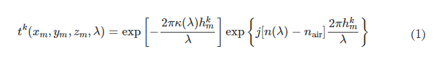
where n(λ) and κ(λ) are the refractive index and the extinction coefficient of the diffractive layer material, respectively; these correspond to the real and imaginary parts of the complex-valued refractive index n~(λ) , i.e., n~(λ)=n(λ)+jκ(λ) (34). For the diffractive unidirectional imager validated experimentally at λ = 0.75 mm, the values of n~(λ) are measured using a terahertz spectroscopy system to reveal n(λ) = 1.700 and κ(λ) = 0.017 for the 3D printing material that we used. The same refractive index value n(λ) = 1.700 is also used in all the diffractive imager models used in our numerical analyses with κ = 0. hkm denotes the thickness value of each diffractive feature on a layer, which can be written as
where hlearnable refers to the learnable thickness value of each diffractive feature and is confined between 0 and hmax. The additional base thickness, hbase, is a constant that serves as the substrate (mechanical) support for the diffractive layers. To constrain the range of hlearnable, an associated latent trainable variable hv was defined using the following analytical form

where Sigmoid(hv) is defined as
Note that before the training starts, hv values of all the diffractive features were initialized as 0. In our implementation, hmax is chosen as 1.07 mm for the diffractive models that use λ = 0.75 mm so that the phase modulation of the diffractive features covers 0 to 2π. For the diffractive imager model that performs wavelength-multiplexed unidirectional imaging, hmax was empirically selected as 1.6 mm, still covering 0 to 2π phase range for both wavelengths (λ1 = 0.75 mm and λ2 = 0.85 mm). The substrate thickness, hbase, was assumed to be 0 in the numerical diffractive models and was chosen as 0.5 mm in the diffractive model used for the experimental validation. The diffractive layers of a unidirectional imager are connected to each other by free space propagation, which is modeled through the Rayleigh-Sommerfeld diffraction equation (33, 49)

where fkm(x,y,z,λ) is the complex-valued field on the mth pixel of the kth layer at (x, y, z), which can be viewed as a secondary wave generated from the source at (xm, ym, zm), r=(x−xm)2+(y−ym)2+(z−zm)2−−−−−−−−−−−−−−−−−−−−−−−−−−−√ , and j=−1−−−√ . For the kth layer (k ≥ 1, assuming that the input plane is the 0th layer), the modulated optical field Ek at location (xm, ym, zm) is given by
where S denotes all the diffractive features located on the previous diffractive layer. In our implementation, we used the angular spectrum approach (33) to compute Eq. 6, which can be written as
where F and F −1 denote the 2D Fourier transform and the inverse Fourier transform operations, respectively, both implemented using a fast Fourier transform. H(xn, yn, zm − zn, λ) is the transfer function of free space
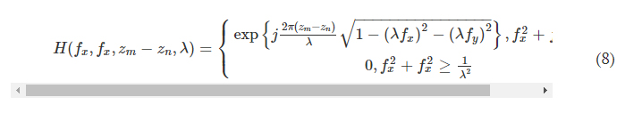
where fx and fy represent the spatial frequencies along the x and y directions, respectively.
Training loss functions and image quantification metrics
We first consider a generic form of a diffractive unidirectional imager, where the image formation is permitted in one direction (e.g., A → B), and it is inhibited in the opposite direction (e.g., B → A) at a single training wavelength, λ. The training loss function for such a diffractive unidirectional imager was defined as
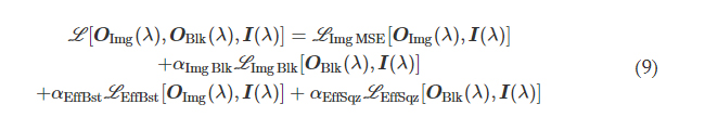
where I(λ) stands for the input image illuminated at a wavelength of λ and OImg(λ) and OBlk(λ) denote the output images in the forward and backward directions, respectively. All the input and output images have the perspective of the illumination beam direction, flipping them left to right as one switches the illumination direction, A → B or B → A. L ImgMSE penalizes the normalized MSE between the OImg(λ) and its ground truth, which can be written as
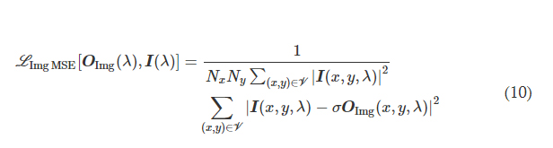
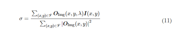
where *(x, y, λ) indexes the individual pixels at spatial coordinates (x, y) and wavelength λ and V denotes the defined FOV that has Nx × Ny pixels at the input or output plane. σ is a normalization constant used to normalize the energy of the diffractive output, thereby ensuring that the computed MSE value is not influenced by the errors arising from the output diffraction efficiency (50), and it is given by the following expression
L EffBst is used to improve the output diffraction efficiency along the imaging direction (e.g., A → B), which is defined as
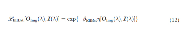
where η(·) is the output diffraction efficiency of the diffractive unidirectional imager and βEffBst is an empirical weight coefficient, which was set as 1.0 during the training of all the diffractive models. η was defined as

L ImgBlk is defined to penalize the structural resemblance between the input image and the diffractive imager output along the image blocking direction (e.g., B → A)

where PCC stands for the Pearson correlation coefficient, defined as

L EffSqz in Eq. 9 is used to penalize the output diffraction efficiency in the backward direction
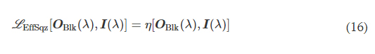
αImgBlk, αEffBst, and αEffSqz in Eq. 9 are the empirical weight coefficients associated with L ImgBlk, L EffBst, and L EffSqz, respectively. We denote the diffractive unidirectional imager output images for A → B and B → A as OA→B(λ) and OB→A(λ), respectively. For the diffractive unidirectional imaging models that were trained using a single illumination wavelength (e.g., in Figs. 2 and 7), the image formation is set to be maintained in the forward direction (A → B) and inhibited in the backward direction (B → A), i.e., OImg(λ) = OA→B(λ) and OBlk(λ) = OB→A(λ). Therefore, the loss function for training these models can be formulated as
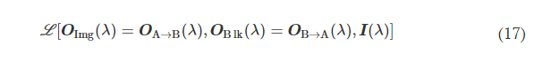
where L (·) refers to the same loss function defined in Eq. 9. During the training of the unidirectional imager models with five diffractive layers and a single training wavelength channel, the empirical weight coefficients αImgBlk, αEffBst, and αEffSqz were set as 0, 0.001, and 0.001, respectively; during the training of the other model with three diffractive layers used for the experimental validation, the same weight coefficients were set as 0, 0.01, and 0.003, respectively.
For the wavelength-multiplexed unidirectional diffractive imager model shown in Fig. 9, at λ1, the image formation is permitted in the direction A → B and inhibited in the direction B → A, whereas at λ2, the image formation is permitted in the direction B → A and inhibited in the direction A → B, respectively; i.e., OImg(λ1) = OA→B(λ1), OBlk(λ1) = OB→A(λ1), OImg(λ2) = OB→A(λ2), and OBlk(λ2) = OA→B(λ2). Accordingly, we formulated the loss function used for training this model as
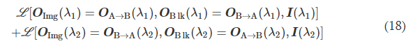
where L (·) refers to the loss function defined in Eq. 9. During the training of this model, the weight coefficients αImgBlk, αEffBst, and αEffSqz were empirically set as 0.0001, 0.001, and 0.001, respectively.
For quantifying the imaging performance of the presented diffractive imager designs, the reported values of the output MSE, output PCC, and output diffraction efficiency were directly taken from the calculated results of L ImgMSE, PCC, and η, respectively, revealing the averaged values across the blind testing image dataset. When calculating the power distributions of different optical modes within the diffractive volume, the power percentage of the output FOV modes takes the same value as η, and the power percentage outside the output FOV is computed by subtracting the total power integrated within the output image FOV from the total power integrated across the entire output plane. The power in the absorbed modes is calculated by summing up the power loss before and after the optical field modulation by each diffractive layer. After excluding the power of the above modes from the total input power, the remaining part is calculated as the power of the unbound modes.
Training details of the diffractive unidirectional imagers
For the numerical models used here, the smallest sampling period for simulating the complex optical fields is set to be identical to the lateral size of the diffractive features, i.e., ~0.53λ for λ = 0.75 mm. The input/output FOVs of these models (i.e., FOV A and B) share the same size of 44.8 by 44.8 mm2 (i.e., ~59.7λ × 59.7λ) and are discretized into 28 by 28 pixels, where an individual pixel corresponds to a size of 1.6 mm (i.e., ~2.13λ), indicating a four-by-four binning performed on the simulated optical fields.
For the diffractive model used for the experimental validation of unidirectional imaging, the sampling period of the optical fields and the lateral size of the diffractive features are chosen as 0.24 and 0.48 mm, respectively (i.e., 0.32λ and 0.64λ). This also results in a two-by-two binning in the sampling space where an individual feature on the diffractive layers corresponds to four sampling space pixels that share the same dielectric material thickness value. The input and output FOVs of this model (i.e., FOV A and B) share the same size of 36 by 36 mm2 (i.e., 48λ × 48λ) and are sampled into arrays of 15 by 15 pixels, where an individual pixel has a size of 2.4 mm (i.e., 3.2λ), indicating that a 10-by-10 binning is performed at the input/output fields in the numerical simulation.
During the training process of our diffractive models, an image augmentation strategy was also adopted to enhance their generalization capabilities. We implemented random translation, random up-to-down, and random left-to-right flipping of the input images using the transforms.RandomAffine function built-in PyTorch. The translation amount was uniformly sampled within a range of [−10, 10] and [−5, 5] pixels in the diffractive unidirectional imager models used for numerical analysis and the model used for the experimental validation, respectively. The flipping operation is set to be performed at a probability of 0.5.
All the diffractive imager models used in this work were trained using PyTorch (v1.11.0, Meta Platforms Inc.). We selected AdamW optimizer (51, 52), and its parameters were taken as the default values and kept identical in each model. The batch size was set as 32. The learning rate, starting from an initial value of 0.03, was set to decay at a rate of 0.5 every 10 epochs, respectively. The training of the diffractive models was performed with 50 epochs. For the training of our diffractive models, we used a workstation with a GeForce GTX 1080Ti graphical processing unit (Nvidia Inc.) and Core i7-8700 central processing unit (Intel Inc.) and 64 GB of RAM, running Windows 10 operating system (Microsoft Inc.). The typical time required for training a diffractive unidirectional imager is ~3 hours.
Vaccination of the diffractive unidirectional imager against experimental misalignments
During the training of the diffractive unidirectional imager design for experimental validation, possible inaccuracies imposed by the fabrication and/or mechanical assembly processes were taken into account in our numerical model by treating them as random 3D displacements (D) applied to the diffractive layers (53). D can be written as

where Dx and Dy represent the random lateral displacement of a diffractive layer along the x and y directions, respectively, and Dz represents the random perturbation added to the axial spacing between any two adjacent layers (including diffractive layers, input FOV A, and output FOV B). Dx, Dy, and Dz of each diffractive layer were independently sampled based on the following uniform (U) random distributions