Reversible electrochemical pH modulation in thin-layer compartments using poly(aniline-co-o-aminophenol)
by Alexander Wiorek, Chen Chen, María Cuartero and Gastón A. Crespo
Abstract: The analysis of many environmental and clinical samples requires the modification of the original pH, which is conventionally carried out by manual/automatic addition of acid, base, or buffering reagents. In the case of decentralized measurements, often, this approach is not plausible. Instead, reagentless alternatives, such as electrochemically activated in-situ pH adjustments, are suitable. Herein, we present a method for electrochemical, reversible pH modulation of thin-layer samples (<100 µm thickness) using the co-polymer poly(aniline-co-o-aminophenol) (PANOA). The PANOA’s electropolymerization strategy was optimized considering the proton exchange properties in the final material. Thus, limiting the maximum anodic potential to 0.85 V and with the number of cyclic scans being ≤150), the optimal pH modulation capabilities were observed. The reversible proton exchange properties of PANOA were quantified by monitoring the pH inside the thin-layer sample (volume of 0.6 µL), which was defined by a 3D-printed microfluidic cell and a pH-sensor placed in a face planar configuration to the PANOA film. A pH value in the range of 2–4 can repeatably be reached in the samples in 3 min, purely by an electrochemical means and without the addition of external reagents. The concept has been demonstrated to acidify samples at environmental pH (artificial samples and Seawater). The outcomes suggest that the family of polyaniline-co-polymers are interesting to be explored and utilized for electrochemically based pH modulation strategies, if careful considerations are taken regarding their electropolymerization process. Overall, such materials could contribute to the development of continuous, decentralized measuring devices requiring acidification for the formal detection of environmental markers, such as nutrients, carbon species speciation and alkalinity, among others.
Keywords: poly(aniline-co-o-aminophenol); polyaniline; PH-modulation; thin-layer electrochemistry; microfluidics
We kindly thank the researchers at KTH Royal Institute of Technology for this collaboration, and for sharing the results obtained with their system.
1. Introduction
The modulation of sample pH is essential in many applications, ranging from analysis and separation of aminoacids [1] to the potentiometric determination of water hardness [2]. In environmental analysis, the use of acid to lower sample pH is necessary before the detection of relevant markers. For example, the detection of phosphate is inherently reliant on the formation of a complex with molybdate (phosphomolybdate), which can be detected optically and/or electrochemically at pH 2 or lower [3], [4]. Another environmentally relevant parameter that requires acid addition (i.e., acid-base titration) for its quantification is alkalinity (typically a pH of 3–4.5 is needed) [5]. Overall, the requirement for acid addition restricts these measurements to centralized laboratories, although on-site or in-situ operation using automatic analyzers has become popular over recent years. While these have helped increasing the frequency of data acquisition for phosphate and alkalinity [6], [7], [8], [9], macronutrients [10] and formaldehyde detection [11], they require waste storage tanks and sometimes, sample dilution before/during the operation, which may cause additional uncertainties in the provided outcomes. To circumvent these drawbacks, light- or electrochemical-driven methodologies for pH modulations could be beneficial instead of reagents additions.
It is possible that the most explored method for pH modulation is the one based on water-splitting at an electrode surface, generating either protons or hydroxide ions [12]. Utilizing a constant applied current or potential, which tends to be very high (ca. 1 mA/cm2 and 2 V), in a thin-layer sample (thickness <100 µm), the pH can be exhaustively shifted in the entire volume. The concept was demonstrated by Van der Schoot et al., showing titrations where the generated charge was used to calculate the moles of acid/base delivered to the sample [12], [13]. Later on Steininger et al. reported on the determination of the sample buffer capacity by measuring the dynamic pH change in the sample generated from water splitting at both the working and counter electrodes, using chemical imaging [14]. Overall, water splitting is indeed an efficient method for adjusting sample pH, but the drastic conditions it requires could lead to undesired side reactions at the electrode surface.
Solid materials presenting proton-coupled redox reactions have proven certain advantages over water splitting for acidification purposes because proton delivery to the sample is possible at low potentials. Balakrishnan et al. showed that 4-aminothiolphenol covalently attached to an electrode surface could shift the pH under electrochemical control in nL volumes for up to 100 reversible cycles [15]. The oxidation of the compound involves a proton exchange: amines are converted into imines in the potential window from 0.65 to 0.8 V. Yet, the proton release capacity shown by this approach is expected to be enough only for nL-volume samples, because of the finite amount of active compound that can be attached to the electrode’s surface. Our group has demonstrated that polyaniline (PANI) is an excellent material for electrochemical pH modulation at even softer potentials than amines (0.2–0.4 V) [16], [17]. This has been used for thin-layer samples acidification coupled to the detection of alkalinity and phosphate [17], [18], [19], as well as chemical imaging of buffer capacity [20], dissolved inorganic carbon (DIC), and carbonate alkalinity [21] in environmental samples. In these works PANI showed suitability for being used for several weeks as long as it is regenerated in acidic solution (10 mM H2SO4) between each acidification usage [22]. Notably, the redox activity and proton release from PANI is not reversible above pH 4–5.
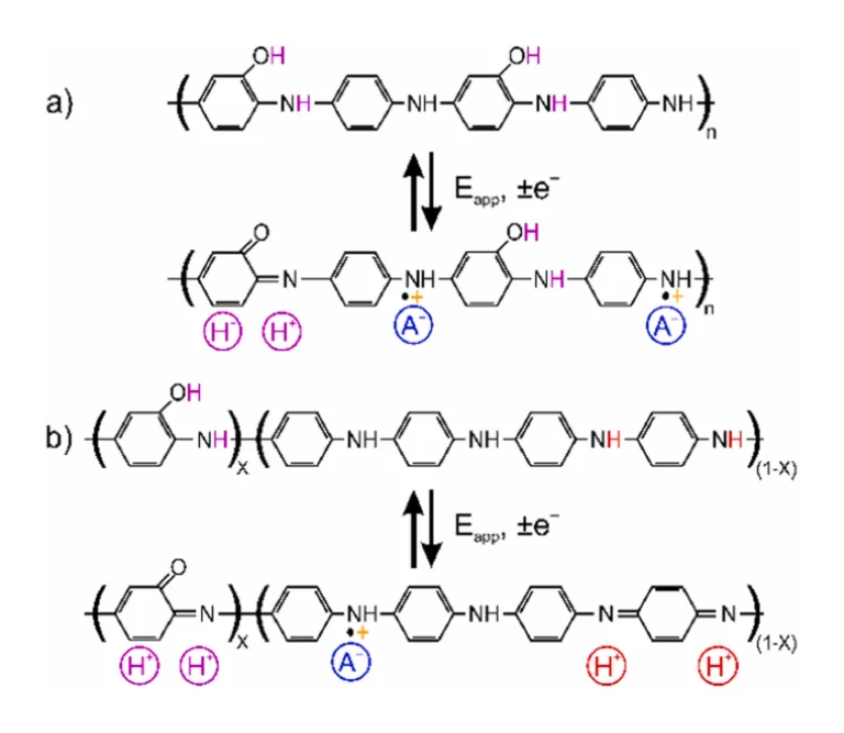
Other PANI-like materials (i.e., co-polymers or polymers containing aniline backbone) could be also of interest, which may be electroactive at higher pH. For example, poly(aniline-co-o-aminophenol) (PANOA), a co-polymer of aniline and o-aminophenol, is an electrochemically active material presenting reversibility at environmental pH values. Mu and coworkers were pioneers investigating the PANOA electropolymerization [23], reporting the structure and redox mechanism as presented in Scheme 1a. The o-aminophenol unit in the PANOA structure allows for reversible redox and proton exchange in solutions up to a pH of 9–10 [23], [24]. In addition, it exhibits anion-exchange properties [25], [26]. The reversibility of PANOA has been attributed to the conversion between the phenolic group (reduced state) and the quinone group (oxidized state) in its backbone. Another suggestion of the PANOA structure and its redox mechanism found in the literature is presented in Scheme 1b, where each o-aminophenol unit is separated by larger PANI-like segments [24], [27]. Here the proton exchange is additionally associated to these segments in the co-polymer. However, because of the poor reversibility of the proton exchange from the amine-imine redox reaction, less efficient proton exchange reversibility at environmental pH is expected than that of the phenol-quinone reaction.
Interestingly, PANOA’s redox activity at physiological and environmental pH values has been crucial for its implementation as a transducer in biosensors and heavy metal sensors [28], [29], among others. In these cases, PANOA was claimed to be superior to PANI in terms of redox activity at physiological pH. However, to the best of our knowledge, the use of PANOA for pH modulation of samples has not been investigated yet, in contrast to PANI [16], [17], [18], [19], [20], [21]. Herein, the use PANOA for reversible proton exchange in thin-layer samples is investigated. PANOA was characterized with both spectroelectrochemistry and thin-layer electrochemistry coupled to in-situ pH sensing. Our experiments revealed the analytical potential regarding further sensing in artificial and real samples that needs for acidification prior to such a detection.
2. Experimental section
2.1. The microfluidic cell and experimental setup of pH modulation in thin-layer samples
The microfluidic thin-layer cell was designed in AutoCAD 2022 (Autodesk) and printed using a Profluidics 285D 3D-printer and Clear Microfluidics Resin V7.0a (CADworks3D). The electrode configuration is presented in Fig. 1a, with a cell schematic shown in Fig. 1b. The cell has an inlet and outlet to allow sample exchange. The outlet additionally contains a pseudo reference/counter electrode (Ag/AgCl wire, RE1/CE1) that is to be connected to the potentiostat. The cell includes a second reference electrode (Ag/AgCl wire, RE2) connected to the potentiometer. Such electrode was inserted into a separate opening present in the cell (the hole with the wire inside was sealed with the 3D-printing resin by curing it with UV-light for 30 s). The center of the cell had a 10-mm-diameter hole to allocate the two electrodes functioning as the acidification actuator (WE1: PANOA) and the pH sensor (WE2: PANI), creating a thin-layer gap sandwiched between them (<100 µm in thickness). Thus, two Au electrodes with a diameter of 3 mm (model 6.09395.034, Metrohm Nordic) were differently modified with PANOA (the working electrode, WE1, in the potentiostat) and PANI (the working electrode, WE2, in the potentiometer), being positioned in such a way that their areas faced each other, being separated by a 90-µm-thick double adhesive tape (RS Online, stock no: 555–033) that was placed on the edges of the electrodes.
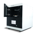
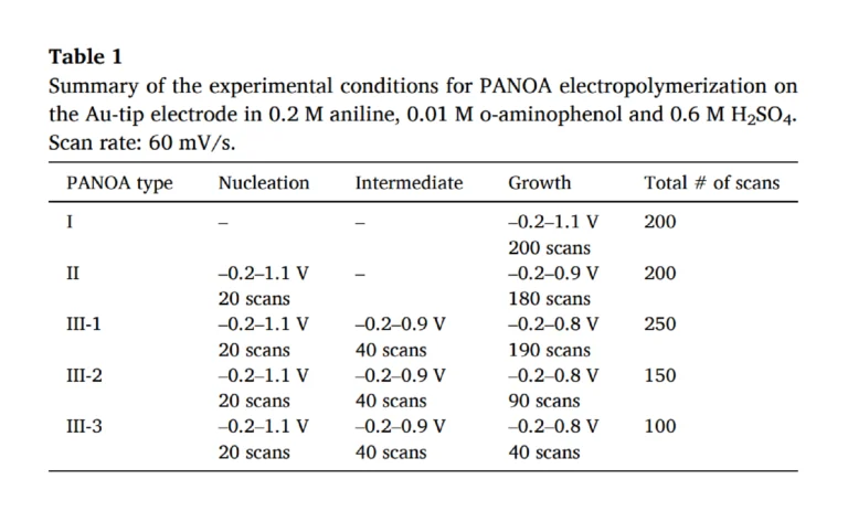
As the PANOA never exceeded a thickness of 10 µm (lower limit of the caliber used for the measurement) this spacer was used for all experiments involving PANOA-based acidifications, providing a configuration with a sample volume of ca. 0.6 µL. The optimized PANOA (as described below; Table 1) was electropolymerized over three different potential windows in succession for cyclic voltammetry (CV); –0.2–1.1 V, –0.2–0.9 V and –0.2–0.8 V, all with a scan rate of 60 mV/s. The PANI-based pH sensor was prepared as optimized elsewhere (–0.05–1.05 V for 10 scans at 100 mV/s) [17]. The pH sensor was calibrated using standards of pH 9.0–1.8 (0.1 M NaCl as background electrolyte; details in the supporting information) inside the microfluidic cell. A typical calibration profile is shown in Figure S1.
Notably, the sample to be acidified is sandwiched between the two electrodes, being confined to a thin-layer domain. This guarantees no mass transport limitation along the sample thickness [30]. In this context, our group has published a model based on the finite element approach to describe the electrochemically controlled release of ions (e.g., H+) from a redox-active film (such as PANOA or PANI) into a sample confined to a thin-layer spatial domain [19]. Calculations were found to rather agree with the experimental results regarding the sample thickness influence on the mass transport regime. On the other hand, the pH achieved in the sample plug after the acidification (i.e., once the needed applied potential stops) may be affected by the lateral diffusion of the rest of the sample contained in the microfluidic system. To confirm that this was not the case, an extra step consisting of the pH recording for some time after acidification ceased was added to the experimental protocol (see below). It is here anticipated that we observed that the pH value achieved through the acidification was maintained.
2.2. Instrumentation
All the electrochemical experiments were performed using a PGSTAT204 Autolab potentiostat (Metrohm Nordic AB) and the Nova 2.1.6 software. The pH sensor was operated by measuring the electromotive force (emf) with a high input impedance (1015Ω), Lawson labs EMF16 Interface (Lawson Laboratories, Inc.). In the spectroelectrochemistry experiments, absorbance spectra were collected using an Avantes ULS2048CL spectrometer with AvaLight-DHc as light source (Avantes) coupled with fiber optics (M92L01, Thorlabs). The pH of the standards used for the calibration of the pH sensor were adjusted using 1 M HCl or 1 M NaOH and a 914 pH/Conductometer from Metrohm (6.0228.000).
3. Results and discussion
The concept and working mechanism herein investigated for PANOA-based acidification of thin-layer samples is illustrated in Fig. 2. The principle is based on a thin-layer sample sandwiched between the source of protons (PANOA) and a potentiometric pH sensor, everything configured in a microfluidic cell. The sample is introduced by means of a peristaltic pump. When the sample plug enters the thin-layer space between the PANOA and the pH sensor, the pump is stopped. The pH of the sample is monitored by the sensor, providing a value representing the initial sample pH. The pH is expected to be stable and determined by the buffer(s) concentration(s) (Fig. 2, left). Then, when PANOA is electrochemically activated by an applied potential, it converts into its higher oxidation state, which involves transforming the phenolic groups of the o-aminophenol units in the co-polymer backbone into quinones [23], [28]. Additionally, some conversion of amines into imines may also occur [24]. Both of these structural changes trigger a release of protons from the PANOA to the thin-layer sample, which converts any base (B–) into its conjugated acid (HB), breaking first the buffer capacity and resulting later in the decrease of the sample pH (Fig. 2, right).
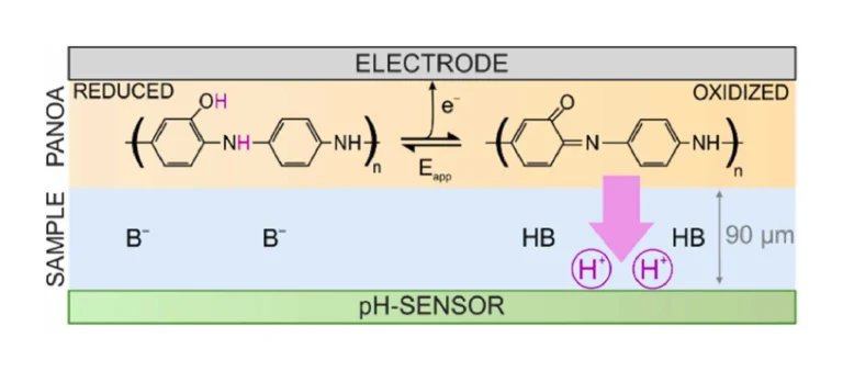
Because of the confined space for the sample, the protons will be largely retained as they can only laterally diffuse in the thin layer, consequently maintaining the lowered sample pH for extended times even after the potential step is finished. Then, by applying a negative potential step to the PANOA, protons in the sample are expected to be re-inserted into the polymer backbone based on its reversible redox mechanism. Thus, in an ideal case, proton exchange with the sample is achievable over numerous cycles. This process, which involves changes in the sample pH, can be followed by the pH sensor placed on the opposite side of the thin layer sample and facing the PANOA. Importantly, once the working mechanism underlying the reversible PANOA-based sample acidification is demonstrated, the pH sensor can be replaced with another sensor (i.e., electrochemical or optical) capable of measuring a pH sensitive analyte, such as a CO2 optode for DIC detection [21], voltammetric sensor for phosphate detection [18], and potentiometric sensors for anions [31], among others.
According to previous findings by Mu et al. and Holze et al., PANOA’s final structure depends largely on the ratio of monomers (aniline and o-aminophenol) involved in its synthesis [23], [24], [32], [33]. As such, if the aniline:o-aminophenol ratio is too high, a more PANI-like structure is expected because of low accessibility of o-aminophenol in the monomer solution [32]. However, when the aniline:o-aminophenol concentration ratio becomes too low, it inhibits the growth of PANOA [23]. Herein, a ratio of 20:1 aniline:o-aminophenol (200:10 mM) in 0.6 M H2SO4 was used for the PANOA electropolymerization, which has been demonstrated to be an adequate condition for producing films that are electroactive at environmental pH values [23]. First, we set out to characterize PANOA using spectroelectrochemical studies, followed by tuning the voltammetric parameters according to its proton exchange properties in the thin-layer cell.
3.1. Spectroelectrochemistry investigation of PANOA
To verify the formation of the PANOA, this was electropolymerized on a transparent ITO electrode while simultaneously recording the absorbance. For this purpose, the experimental setup was based on the spectroelectrochemical cell used in our previous works [16], [34]. Initially, the electropolymerization was performed by CV (from –0.2–1.1 V at 60 mV s–1 for 20 scans). Some selected scans are presented in Fig. 3a. Notably, the results are analogous to previous studies reporting PANOA formation at the same potential window [23], [35], implying the successful formation of the co-polymer.
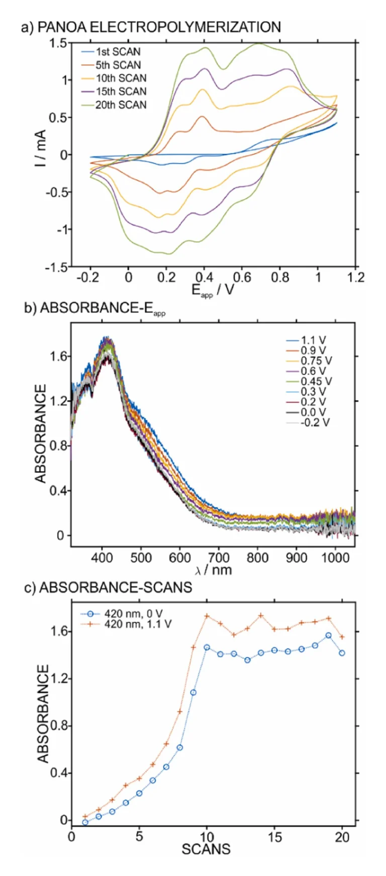
Several waves can be observed in the anodic part. Two peaks at 0.25 and 0.38 V, which have been ascribed to the first oxidation state of the polymer chain during its growth [23], [36], including anion insertion into the film [26]. Then, a small peak is observed at ca 0.7 V during the first scan, which corresponds to the oxidation of the phenolic group in acidic conditions [23]. Also, two partly overlapping peaks are found at 0.8–0.9 V, which are ascribed to the second oxidation state of the polymer [26] as well as oxidations of the monomers [23], [26]. After eight scans, two peaks appeared at 0.55 and 0.63 V. Despite these being observed in previous works [23], [37], the origin is not clear yet, resulting in incomplete explanations. Notably, by analogy to PANI and considering that both polymers (PANI and PANOA) present a similar structure, this peak likely originates from degradation products in the hydrolysis of imines in the polymer backbone [38]. In the cathodic part, in the potential window from 0.8 to 0.9 V (i.e., in the region of the second oxidation state of the polymer), there is a small peak at approximately 0.65 V. Then, the first oxidation state relates to three peaks in the potential range from –0.1–0.3 V, instead of the two peaks presented in the anodic part.
The spectra connected to the anodic part of the final scan of the electropolymerization process are presented in Fig. 3b. Different absorbance bands are absorbed in the region from 380 to 530 nm, with small increases in magnitude with the applied potential. This effect is in accordance with previous results about PANOA electropolymerization [33], confirming the formation of the co-polymer. To further analyze the spectroelectrochemical results, the change in absorbance at the absorbance maximum (420 nm) during the anodic scans at PANOA’s reduced state (0 V) and its fully oxidized state (1.1 V) versus the number of scans are presented in Fig. 3c. It was observed that the absorbance at 420 nm increased until the 10th scan, whereafter it remained almost constant. The full spectra during the growth of the polymer are provided in Figure S2. Additionally for each individual scan, the oxidized state always presented a higher absorbance. This behavior contrasts with that found for the current in the voltammetric peaks, where all peaks gradually increased over the 20 scans. Overall, the result in the absorbance suggested that further growth of the molecular structure corresponding to the 420 nm band does not occur after the 10th scan. Interestingly, this ceased increase in absorbance coincides with the emergence of the anodic peak at 0.55 V.
3.2. Optimization of PANOA fabrication via electropolymerization
After the spectroelectrochemical measurements and for further experiments, the ITO electrode substrate was replaced by the Au electrode tip to improve the mechanical stability of the created film. The total number of scans of in the electropolymerization process was increased from 20 (for ITO) to 100–250 for the Au-electrodes. Thus, thicker films were expected in the Au than in the ITO substrate, aiming for a more efficient acidification strategy (i.e., the film will contain a higher number of protons to be delivered from the PANOA to the sample) considering the proof of concept in real water samples [16], [17]. Additionally, having identified in the spectroelectrochemistry results that there is a peak at 0.55 V surely related to the polymer degradation, an even more improved efficiency for the PANOA-sample proton exchange was expected by decreasing the maximum anodic potential used in the CV during electropolymerization. Effectively, thanks to preliminary experiments based on PANI electropolymerization by decreasing the upper limit of the CV potential window from 1.2 to 0.75 V (Figure S3a), it was found out that lowering the anodic potential below 0.9 V translated into the disappearance of the peak at 0.55 V with consecutive scans (Figure S3b).
Next, a systematic study was performed to understand if avoiding the degradation peak at 0.55 V led to an improved electrochemical performance for PANOA films. In essence, we investigated the effect of the upper potential in the growth window for PANOA electropolymerization while keeping constant the scan rate (60 mV/s) and the initial potential (–0.2 V) on the obtained CV (i.e., number of peaks and the related current). The experimental setup used was based on a three-electrode configuration in a beaker. The electropolymerization conditions are listed in Table 1 and the generated PANOA films were classified as PANOA types I, II and III. As justified below, the synthesis of PANOA type II included an initial nucleation step and that for PANOA type III an additional intermediate step that led to improved film growth. For PANOA type III, the number of scans in the growth part was changed, giving rise to the subclasses 1, 2 and 3. Overall, the CVs on Au shared similar peaks as those on the ITO-electrode (Fig. 4).
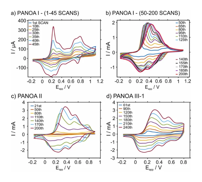
The trend over the first 45 scans of PANOA type I is illustrated in Fig. 4a. The following differences with the results observed for the ITO electrode. Were found. The first peak shifted to slightly lower potentials (0.23 V) and is initially lower in current magnitude than the second peak at 0.38 V. After 30 scans, the peak at 0.23 V becomes the most prominent. The second oxidation state associated to the two peaks at 0.63 V and 0.75 V, which also has been attributed to PANOA growth [23], exhibited a higher current than the first oxidation state (peaks at 0.23 and 0.38 V) until the 35th scan. The peak at 0.55 V did not appear until the 45th scan, indicating that no degradation occured before this point.
Fig. 4b presents the growth of PANOA type I from the 50th to the 200th scan. After the 65th scan the peaks at 0.23 and 0.38 V start to overlap and are no longer distinguishable, while the peaks at 0.63 and 0.75 V start to overlap with the peak at 0.55 V. Notably, PANOA of type I did not exhibit an increase in peak currents after 150 scans, whereafter the peaks shifted towards higher potentials. This can be likely scribed to two origins; i) an increase in film thickness providing additional resistance [17], and/or ii) the fact that the peak at 0.55 V becomes more pronounced between the 50th and 200th scans may result in film degradation and hence, impaired film conductivity [38], [39].
For PANOA of type II, the anodic limit was lowered to 0.9 V compared to type I, attempting to avoid the peak at 0.55 V. However, the peaks’ currents were found to increase very slowly (data not shown) using this potential window alone, indicating a slow film growth. Thus, a nucleation step of 20 scans between –0.2 and 1.1 V was implemented prior to the regular CV protocol. In such a case, the peak at 0.55 V was not observed (Figure S4a). Subsequently 180 scans between –0.2 and 0.9 V were adapted (Fig. 4c) for a total of 200 scans considering the entire procedure. This was still not sufficient to remove the peak at 0.55 V at the end of electropolymerization. However, PANOA II accumulated a final charge of 21.0 mC, which was more than a three-time-increase compared to PANOA Type I (6.1 mC). Thus, although the potential window was decreased, the amount of charge inserted into PANOA was increased.
Then, the potential window for the CV was fixed from –0.2–0.8 V for PANOA III-1, III-2, and III-3 after the established nucleation (from –0.2–1.1 V, 20 scans). Notably, preliminary tests applying this protocol provided a very slow growth of PANOA (i.e., slow current increase with subsequent scans). Thus, an intermediate step was implemented: from –0.2–0.9 V for 40 scans. Within the 40 scans, the peak at 0.55 V has not appeared yet (Figure S4b). Thus, the third strategy for the PANOA synthesis comprised three steps: i) nucleation step (CV from –0.2–1.1 V, 20 scans), ii) intermediate step (CV from –0.2–0.9 V, 40 scans), and iii) growth step (CV from –0.2–0.8 V for 190, 90 or 40 scans to obtain PANOA III-1, III-2, and III-3, respectively). The progression of the final step is presented in Fig. 4d. The main differences considering PANOA I and II (Fig. 4a-c) is that the peak for the second oxidation state (0.74 V) is still visible at the end of the electropolymerization.
This becomes more evident when comparing the last CV in the growth part for PANOA I, II and III (of any subclass), which are displayed in Fig. 4a-d and Figure S4c. It can be observed that PANOA III-1 (with the higher number of scans in the growth part) presented the peak at 0.74 V corresponding to the second oxidation state, and the peak at 0.33 V (Fig. 4d) did not shift as much as it does in PANOA I and II, which suggests a lower degree of degradation in PANOA III. Lowering the upper potential in the growth window further could perhaps be an option to avoid the peak at 0.55 V completely but would also decrease the rate of growth.
Comparing PANOA III-1, III-2 and III-3, the one that presented final current levels much closer to that displayed for PANOA I and II was PANOA III-1. Moreover, an extension in the number of scans from 200 to 250 for PANOA III-1 was considered because, unlike PANOA I and II, the voltammetric peaks were still increasing for each scan after 200 scans. This increase in current magnitude for each scan was suggesting that the film thickness was still growing. On the other hand, PANOA Type III-2 and III-3 presented lower peak currents at the end of their formation, but the shape of the CV are more similar to that claimed as characteristic for PANOA [23], [35], with the peak at 0.55 V being far less pronounced than in the case of all the other PANOA types.
Overall, it can be concluded that limiting the upper potential for the electropolymerization window avoids PANOA degradation to some extent but, at the same time, it restricts the rate of growth (considering the increase in peak currents). Accordingly, the optimal conditions to be selected are expected to be a compromise between degradation and growth effect providing the best proton exchange capacity that can be held by PANOA (i.e., sites to store protons in the co-polymer backbone).
3.3. Investigation of PANOA acidification capacity
To quantify the proton exchange properties of the different PANOA types and the reversibility of the process, we introduced the corresponding PANOA-Au electrode into the microfluidic thin-layer sample cell (Fig. 1), where the sample pH could be continuously monitored by the potentiometric pH sensor. The experimental protocol to induce electrochemical pH modulations in the sample together with the expected readout from the pH sensor are presented in Fig. 5a and b respectively. This consists of: (1) initial reading of the open circuit potential (OCP) by the potentiostat and the potentiometer with the pH sensor; (2) acidification step by applying the +0.4 V for 300 s to the PANOA electrode; (3) passive monitoring step at the OCP for 60 s; and (4) PANOA regeneration step at –0.2 V for 600 s. All these steps were performed in the same sample plug (i.e., with the pump turned off). Importantly, the acidification potential was selected to be 0.4 V to avoid being closer to potentials inducing secondary processes beyond proton release that may contribute to increase the charge released from PANOA and even its degradation. A similar strategy was followed in our previous papers involving PANI [16], [17].
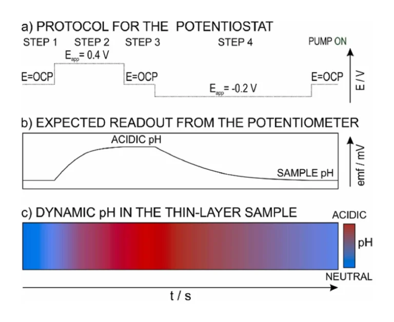
Initially, when no potential is applied in step 1, a constant readout from the potentiometer was expected, which corresponds to the initial pH of the sample. Then in step 2, the PANOA is activated at the +0.4 V for 300 s, triggering the release of protons from the film to the sample. This causes a response from the pH sensor because of the pH shift in the thin-layer sample. Fig. 5c additionally illustrates the dynamic change in pH expected in the sample: from the initial pH to an acidified pH and finally coming back to the initial pH because of the regeneration step. In step 3, the applied potential was switched off and the pH readout was recorded in the thin-layer sample for 60 s, expecting the pH to be constant and equivalent to the level of acidification achieved by the actuator (always that there are not diffusion related uniformities in the process). In step 4, the PANOA is regenerated in the same sample plug: proton uptake from the acidified sample thanks to the application of –0.2 V for 600 s. This step causes the sample pH to return to its original value. Regarding the time of 600 s, according to the pH monitoring in numerous experiments, it was found that shorter times did not allow for a complete regeneration of the PANOA (meaning that the initial sample pH was not recovered), and longer times did not improve the regeneration efficiency. Then, after the regeneration, the peristaltic pump was turned on for 5 – 15 minutes to exchange the sample plug for further experiments.
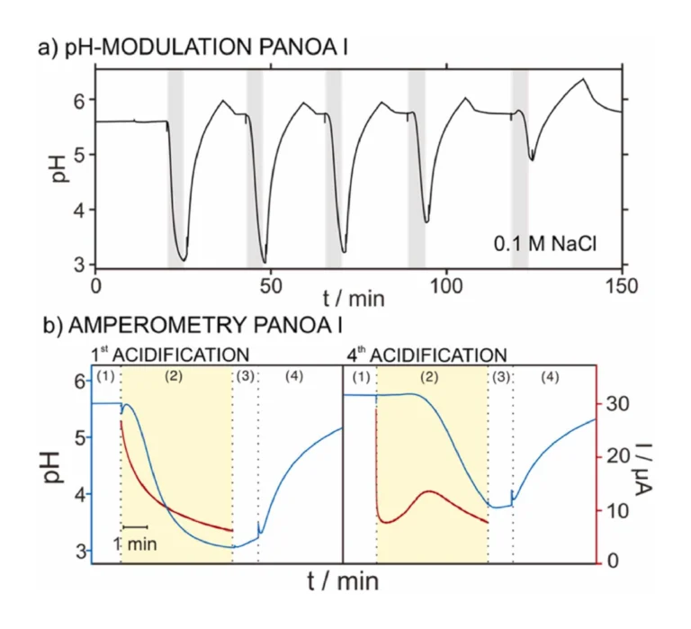
The repeatability of the results provided by this protocol was first tested on PANOA type I in 0.1 M NaCl sample solution, accomplishing five consecutive cycles of pH modulation. Fig. 6a depicts the dynamic pH that was observed. The first three cycles reached an acidified pH of 3.11±0.11; whereafter, a decrease in the acidification capacity was observed (pH of 3.77 and 4.91 for the fourth and fifth acidifications respectively). Notably, this final pH was calculated as the average pH value shown during step 3 (i.e., no applied potential, just measuring the pH for 60 s after acidification, when the sample just holds the acidified pH). This criterion was used through the paper. The described behavior coincided with a progressive change in the current profiles associated to each proton release (Figure S5a, charge of 3.28±0.84 mC). Moreover, the regeneration step for taking up protons was also found to become less efficient in consecutive cycles (Figure S5b, charges of –3.84±0.95). These trends also manifested in an overall decrease in charge for both the delivery and regeneration steps (Figures S5c-d): for the second to fifth cycle of acidification, the charge was decreased from 4.25 mC to 1.80 mC and the decrease was 57.6 %; for the first to fifth cycles of proton uptake process, the charge was decreased from –4.82 mC to –2.2 mC, decrease in 54.3 %. Inspecting the pH acidification with the corresponding current profile for the first and fourth cycles, which are those displaying the biggest differences, some conclusions can be established. As observed in Fig. 6b, the first current transient displayed a Cottrell-like profile, while the fourth one displayed an initial fast decay and then the current slowly increased, therefore displaying a peak. For the first acidification, the decrease in pH was initiated within the first 15 s after activating the potential step. On the other hand, the fourth acidification displayed a considerable delay (ca. 100 s) before a decrease in pH was observed, which interestingly coincided with the peak in the current profile. This may imply that such a peak is closely related to the process of releasing protons from PANOA type I. However, because of the poor repeatability in both the acidification and charge delivery profile (i.e., electrochemical performance), we averted from further studies into this process, because PANOA type I was concluded not suitable for reversible pH modulations.
The results for the repeatability study of PANOA type II are presented in Fig. 7a, revealing ∆pH=2.82±0.06 for eight cycles (ΔpH=2.96±0.18 for the first 3 cycles). Effectively, the overall electrochemical performance was found to improve with respect to PANOA type I, but again showing some differences within increasing number of cycles (Figure S6). As observed in Figure S6a, the current for the first acidification is lower than subsequent pH modulations and displays no peak in the dynamic current profile. The increase in the current magnitude from the first acidification and the latter ones can be explained from a decrease observed in the OCP: 0.080 V for the first and –0.139±0.012 V for the subsequent cycles. In essence, because the potential step is larger from –0.139 V to 0.4 V than from 0.080, more charge is expected to be generated in the PANOA. Despite the mentioned differences in the current profiles, only small variations were found in the corresponding charges (4.69±0.13 mC, excluding the first acidification; Figure S6b). In addition, the pH measured in the regeneration step was found to always return to a pH very close to the initial sample pH, also displaying very similar current profiles and acceptable reproducibility in terms of charge (–4.89±0.20 mC, Figures S6c and S6d).
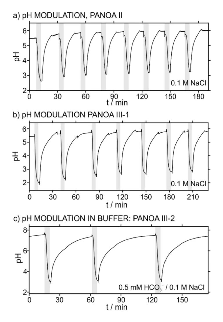
With an acceptable electrochemical and pH modulating performance confirmed for 0.1 M NaCl solution, PANOA type II was further tested in a buffered solution (0.5 mM NaHCO3/0.1 M NaCl). The operational performance in higher, buffered pH is interesting to be evaluated in terms of PANOA usability in environmental waters and physiological conditions. However, it was found that the pH modulation using PANOA type II was not reversible under these conditions (Figure S7). Triplicate measurements revealed a successful first pH modulation, shifting the pH from the initial value of 7.6 to below 4 at the end of the acidification. But, in subsequent pH modulations, the pH was unable to be shifted below 6.5. This motivated the development of the PANOA type III and its subclasses, to provide an electrochemically induced pH actuator that is reversible at higher pH values.
The repeatability of the pH modulation induced by PANOA type III-1 in 0.1 M NaCl was found to be higher and more efficient than PANOA type II when tested in unbuffered conditions. An acidification of ∆pH=3.12±0.19 over seven cycles (Fig. 7b), with charge deliveries of 6.43±0.53 mC and –6.82±0.49 mC for the acidifications and regenerations (Figure S8) were revealed. Moreover, this proper performance was additionally accompanied by an improved repeatability in 0.5 mM NaHCO3 (with 0.1 M NaCl as background electrolyte), reaching final pH values of 3.4, 3.7 and 4.1 in consecutive acidifications (initial pH=7.5; Figure S9a). Yet, the decreasing trend within each subsequent acidification in unbuffered conditions motivated the development of the PANOA type III-2 and type III-3 subclasses, which showed excellent repeatability in buffered media (Fig. 7c and Figure S9b for type III-2 and type III-3, with average charges of 2.66±0.17 mC and 2.92±0.13 mC, respectively).
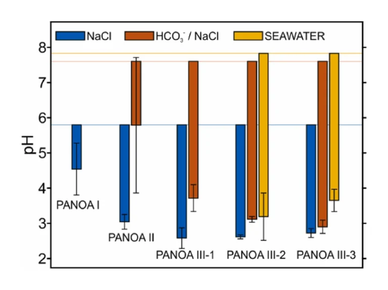
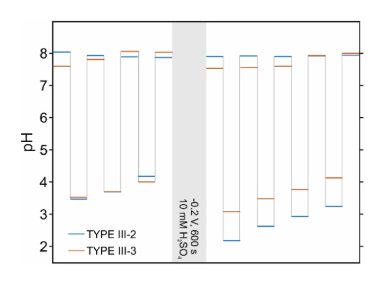
The overall improvement over all tested PANOA types is summarized in Fig. 8 for all tested samples; 0.1 M NaCl (blue), 0.5 mM NaCO3–, and seawater (discussed in detail in the next section). The corresponding pH values are provided in Table S1 in the Supporting Information. The horizontal lines indicate the average starting pH over all measurements for the corresponding samples, the bars extending from the starting pH give the magnitude of the acidification and their average final pH, and the error bars provided the standard deviations for the measurements. Indeed, the subclasses of both PANOA type III-2 and III-3 behaved roughly the same, where both provided improved acidification-capacities and repeatability compared to types I, II and III-1 for both unbuffered (Fig. 8, blue bars) and buffered samples (Fig. 8, orange bars). By comparing the preparation protocols (Table 1) and the CVs in Fig. 4 with the acidification results, the following can be concluded. By limiting the formation of the degradation peak at 0.55 V, the acidification capacity (i.e., decrease in pH) increases, and the repeatability (standard deviation) decreases indicating an improvement in reversibility of the proton release from the PANOA film.
3.4. pH modulation of seawater samples using PANOA as an electrochemically driven actuator
Considering the superior efficiency and reversibility of the proton exchange from the PANOA Type III-2 and Type III-3 compared to the other PANOA types, we further tested their performance in a seawater sample (collected at Torrevieja, Spain, Supporting Information). Three subsequent acidifications/regenerations were tested. Notably, the applied potential was changed to 0.45 V for acidification and –0.15 V for regeneration to adjust for the higher chloride concentration (ca. 0.6 M) in seawater, which shifts the reference potential by approximately 50 mV compared to the artificial samples containing 0.1 M NaCl as the background electrolyte (with or without buffer). The sample’s pHs measured before and after acidification are presented in Fig. 9. The dynamic pH-time profiles are additionally provided in Figure S10. As observed, the acidified sample presented a pH value that increased with the number of cycles, while the pH obtained after the regeneration decreased. Averages values of 3.19±0.67 and 3.67±0.35 were respectively found for PANOA Type III-2 and PANOA Type III-3 (yellow bars Fig. 8), indicating that PANOA III-2 has a slightly higher capacity for acidification than PANOA III-3. Overall, the proton exchange efficiency was mitigated with the number of cycles, an effect that was not noticed in the buffered samples used in the previous section. The higher complexity of the sample matrix together with the higher buffer capacity (alkalinity=2.47±0.04 mM, details in the Supporting Information) may indeed affect the PANOA’s proton exchange properties.
To extend the number of uses of the PANOA film, a more drastic regeneration procedure was investigated. Thus, after the three consecutive pulses, an acid solution (10 mM H2SO4/0.1 M NaCl) was pumped into the cell and a potential of –0.2 V was applied for 600 s. Thereafter, the seawater sample was re-introduced in the microfluidic cell, and four consecutive acidification-regeneration cycles were performed. The regeneration step in acid solution was found to significantly increase the acidification capacity of the PANOA films, which was more pronounced for PANOA Type III-2 than PANOA Type III-3, with final pHs of 2.2, 2.6, 2.9 and 3.2 versus 3.1, 3.5, 3.7 and 4.1.
These results are indeed relevant in view of the further application of the PANOA as an acidification actuator for environmental monitoring purposes. When acid-based regenerations are possible to implement, the use of PANOA Type III-2 is preferred over PANOA III-3 because of its higher acidification capacity. Moreover, it is possible to acidify the sample, run a sensor-based measurement (i.e., with the microfluidic cell integrating an analytical sensor instead of the pH one, which only means to monitoring the acidification-regeneration process in this study), and a regeneration step using the same sample for many successive cycles (at least 4). This option drastically reduces the need for acid solutions compared to traditional manual/automatized acid additions, empowering the greener perspective of the developed concept.
The frequency selected for introducing the acid for regeneration will then depend on the pH threshold required for the analytical application. Other option, which could be adopted depending on the final pH desired in the sample after acidification, is the sole use of the acidified sample for the regeneration. Some pH values to be considered as examples would be 4.5 to detect dissolved inorganic carbon [21], and 4.8 for the total sulfide detection [40], both attainable without using acids in the regeneration step. Although PANOA Type III-2 was found to be capable of lowering the pH more than PANOA Type III-3, the latter generates more charge, as obtained in the integration of the current-time curves (Figure S11). The higher charge output is likely because of that the thinner film avoids the degradation peak (0.55 V), which allows the polymer to maintain its conductivity and capacitance compared to thicker films. Additionally, it is likely that all charge generated does not correspond to protons, but also other processes such as anion-insertion into the PANOA [25], and different relaxation processes of the polymer [41].
3.5. Performance comparison between PANOA- and PANI-based acidification
The use of PANI has been recently demonstrated for the successful reagentless acidification of environmental samples. Thus, we performed a series of additional experiments to compare the performance of PANOA and PANI, investigating the reversibility and efficiency of the proton delivery/uptake from PANI. The PANI film was prepared with previously optimized voltammetric parameters (1.1 V for 10 s, followed by –0.35–0.85 V at 100 mV/s) [17], [18], [19], [20], [21], with 200 scans of electropolymerization (Figure S3b) resulting in a film thickness of ca. 350 µm. The spacer in the electrochemical cell was adjusted to assure that the thin-layer thickness would remain approximately constant and like that used for the PANOA films (details in Section 3 in the Supporting Information). Then, compared to already published investigations with PANI, the acid-based regeneration step normally conducted in 10 mM H2SO4 [17], [18], [19], [20], [21], was substituted using the acidified sample plug, to be comparable with the experimental conditions herein established for PANOA.
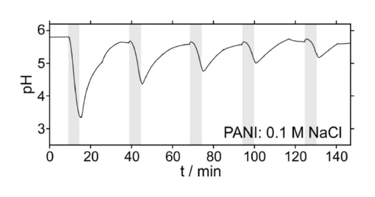
The results for 5 acidification-regeneration cycles are displayed in Fig. 10. A poor reversibility of the proton exchange was observed in 0.1 M NaCl sample solution, with a dramatic decrease in the acidification capacity over the five scans (final pH values of 3.3, 4.4, 4.8, 5.0 and 5.2). Accordingly, PANI exhibited excellent reversibility when regenerated in an acidic solution with a pH lower than 2 (10 mM H2SO4 solution) [16], [17]. The regeneration pH significantly influences the conversion of PANI to its protonated state. In this experiment, using a non-acid-based regeneration step, the lowest achieved pH was 3.3. This pH level was not sufficient to fully convert PANI to its protonated state, demonstrating that non-acid-based regeneration is not suitable to ensure successive acidification. On the other hand, the charge delivered by PANI was found to be ca. 10 times higher than for PANOA, and quite constant over all the pH modulation cycles (26.8±1.4 mC for the acidifications and –32.2±0.35 mC for the regenerations), as observed in Figure S12. This suggested that PANI would indeed be capable of delivering a superior charge compared to PANOA, although all of this charge is not expected to be correlated to the release of protons but also anion-exchange processes [17], [42]. But, if more protons are needed for the specific application, PANI can be grown thicker by increasing the number of scans or subsequently adjusting the potential window during its electropolymerization without observing the degradation peak observed for PANOA (0.55 V) [17], [21]. However, all these strategies will always accompanied by an acid-based regeneration step in contrast to PANOA.
4. Conclusion
An electrochemical method for reversible pH modulations in thin layer samples (<100 µm thickness) was herein presented using the electropolymerized copolymer between o-aminophenol and aniline PANOA. The outcomes demonstrated the relevance of the electropolymerization strategy towards achieving optimal proton-coupled redox properties from the material. Specifically, by limiting the maximum anodic potential to 0.85 V and number of cyclic scans to ≤150, optimal pH modulation capabilities were observed, as quantified by in-situ potentiometric measurements of the pH inside the thin-layer sample (volume of 0.6 µL; defined by a 3D-printed microfluidic cell). It was found that the optimized PANOA film can consistently acidify samples (artificial and real seawater) to pH 2–4 within 3 min by purely electrochemical means and without addition of reagents to the sample. Such a pH is indeed suitable for the sensing of certain environmental markers, such as dissolved inorganic carbon and dissolved inorganic phosphate.
Supplementary material
References
- T. Ueda, R. Mitchell, F. Kitamura, T. Metcalf, T. Kuwana, A. Nakamoto, Separation of naphthalene-2,3-dicarboxaldehyde-labeled amino acids by high-performance capillary electrophoresis with laser-induced fluorescence detection, J. Chromatogr. A 593 (1) (1992) 265–274, https://doi.org/10.1016/0021-9673(92)80295-6.
- M. Müller, M. Rouilly, B. Rusterholz, M. Maj-Zurawska, ˙ Z. Hu, W. Simon, Magnesium selective electrodes for blood serum studies and water hardness measurement, Microchim. Acta 96 (1) (1988) 283–290, https://doi.org/10.1007/BF01236112.
- C. Warwick, A. Guerreiro, A. Soares, Sensing and analysis of soluble phosphates in environmental samples: a review, Biosens. Bioelectron. 41 (2013) 1–11, https://doi.org/10.1016/j.bios.2012.07.012.
- J. Jonca, ´ V. Leon´ Fernandez, ´ D. Thouron, A. Paulmier, M. Graco, V. Garçon, Phosphate determination in seawater: Toward an autonomous electrochemical method, Talanta 87 (2011) 161–167, https://doi.org/10.1016/j.talanta.2011.09.056.
- T. Michałowski, A.G. Asuero, New approaches in modeling carbonate alkalinity and total alkalinity, Crit. Rev. Anal. Chem. 42 (3) (2012) 220–244.
- M.Z. Bieroza, A.L. Heathwaite, Seasonal variation in phosphorus concentration–discharge hysteresis inferred from high-frequency in situ monitoring, J. Hydrol. 524 (2015) 333–347, https://doi.org/10.1016/j.jhydrol.2015.02.036.
- L. Qiu, Q. Li, D. Yuan, J. Chen, J. Xie, K. Jiang, L. Guo, G. Zhong, B. Yang, E. P. Achterberg, High-precision in situ total alkalinity analyzer capable of monthlong observations in seawaters, ACS Sens. (2023), https://doi.org/10.1021/acssensors.3c00552.
- C. Sonnichsen, D. Atamanchuk, A. Hendricks, S. Morgan, J. Smith, I. Grundke, E. Luy, V.J. Sieben, An automated microfluidic analyzer for in situ monitoring of total alkalinity, ACS Sens. 8 (1) (2023) 344–352, https://doi.org/10.1021/acssensors.2c02343.
- R.S. Spaulding, M.D. DeGrandpre, J.C. Beck, R.D. Hart, B. Peterson, E.H. De Carlo, P.S. Drupp, T.R. Hammar, Autonomous in situ measurements of seawater alkalinity, Environ. Sci. Technol. 48 (2014) 9573–9581, dx.doi.org/10.1021/es501615x.
- M. Cuartero, G.A. Crespo, T. Cherubini, N.C.F. Pankratova, F. Massa, M.L.A. M. Tercier-Waeber, J. Scha¨fer, E. Bakker, In situ detection of macronutrients and chloride in seawater by submersible electrochemical sensors, Anal. Chem. 90 (2018) 4702–4710, https://doi.org/10.1021/acs.analchem.7b05299.
- I.-Y. Eom, Q. Li, J. Li, P.K. Dasgupta, Robust hybrid flow analyzer for formaldehyde, Environ. Sci. Technol. 42 (4) (2008) 1221–1226, https://doi.org/10.1021/es071472h.
- B. Van der Schoot, P. Bergveld, An IFSET-based microlitre titrator integration of a chemical sensor-actuator system. Sens. Actuators 8 (1985) 11–22, https://doi.org/10.1016/0250-6874(85)80020-2.
- B. van der Schoot, P. van der Wal, N. de Rooij, S. West, Titration-on-a-chip, chemical sensor–actuator systems from idea to commercial product, Sens. Actuators B 105 (2005) 88–95.
- F. Steininger, S.E. Zieger, K. Koren, Dynamic sensor concept combining electrochemical pH manipulation and optical sensing of buffer capacity, Anal. Chem. 93 (2021) 3822–3829, https://doi.org/10.1021/acs.analchem.0c04326.
- D. Balakrishnan, J. El Maiss, W. Olthuis, C. Pascual García, Miniaturized control of acidity in multiplexed microreactors, ACS Omega 8 (8) (2023) 7587–7594, https://doi.org/10.1021/acsomega.2c06897.
- A. Wiorek, M. Cuartero, R. De Marco, G.A. Crespo, Polyaniline films as electrochemical-proton pump for acidification of thin layer samples, Anal. Chem. 91 (2019) 14951–14959, https://doi.org/10.1021/acs.analchem.9b03402.
- A. Wiorek, G. Hussain, A.F. Molina-Osorio, M. Cuartero, G.A. Crespo, Reagentless acid− base titration for alkalinity detection in seawater, Anal. Chem. 93 (2021) 14130–14137, https://doi.org/10.1021/acs.analchem.1c02545.
- C. Chen, A. Wiorek, A. Gomis-Berenguer, G.A. Crespo, M. Cuartero, Portable all-inone electrochemical actuator-sensor system for the detection of dissolved inorganic phosphorus in seawater, Anal. Chem. 95 (8) (2023) 4180–4189, https://doi.org/10.1021/acs.analchem.2c05307.
- A.F. Molina-Osorio, A. Wiorek, G. Hussain, M. Cuartero, G.A. Crespo, Modelling electrochemical modulation of ion release in thin-layer samples, J. Electroanal. Chem. 903 (2021) 115851, https://doi.org/10.1016/j.jelechem.2021.115851.
- F. Steininger, A. Wiorek, G.A. Crespo, K. Koren, M. Cuartero, Imaging sample acidification triggered by electrochemically activated polyaniline, Anal. Chem. 94 (40) (2022) 13647–13651, https://doi.org/10.1021/acs.analchem.2c03409.
- A. Wiorek, F. Steininger, G.A. Crespo, M. Cuartero, K. Koren, Imaging of CO2 and dissolved inorganic carbon via electrochemical acidification–optode tandem, ACS Sens. (2023), https://doi.org/10.1021/acssensors.3c00790.
- E.M. Genies, A. Boyle, M. Lapkowski, C. Tsintavis, Polyaniline: a historical survey, Synth. Met. 36 (1990) 139–182.
- S. Mu, Electrochemical copolymerization of aniline and o-aminophenol, Synth. Met. 143 (3) (2004) 259–268, https://doi.org/10.1016/j.synthmet.2003.12.008.
- J. Zhang, D. Shan, S. Mu, Chemical synthesis and electric properties of the conducting copolymer of aniline and o-aminophenol, J. Polym. Sci. Part A: Polym. Chem. 45 (23) (2007) 5573–5582, https://doi.org/10.1002/pola.22303. DOI: https://doi.org/10.1002/pola.22303 (acccessed 2023/07/03).
- Y. Zhang, S. Mu, B. Deng, J. Zheng, Electrochemical removal and release of perchlorate using poly(aniline-co-o-aminophenol), J. Electroanal. Chem. 641 (1) (2010) 1–6, https://doi.org/10.1016/j.jelechem.2010.01.021.
- M. Liu, M. Ye, Q. Yang, Y. Zhang, Q. Xie, S. Yao, A new method for characterizing the growth and properties of polyaniline and poly(aniline-co-o-aminophenol) films with the combination of EQCM and in situ FTIR spectroelectrochemisty, Electrochim. Acta 52 (1) (2006) 342–352, https://doi.org/10.1016/j.electacta.2006.05.013.
- Y. Zhang, F. Wen, Y. Jiang, L. Wang, C. Zhou, H. Wang, Layer-by-layer construction of caterpillar-like reduced graphene oxide–poly(aniline-co-o-aminophenol)–Pd nanofiber on glassy carbon electrode and its application as a bromate sensor, Electrochim. Acta 115 (2014) 504–510, https://doi.org/10.1016/j.electacta.2013.10.143.
- S. Mu, Direct determination of arsenate based on its electrocatalytic reduction at the poly(aniline-co-o-aminophenol) electrode, Electrochem. Commun. 11 (7) (2009) 1519–1522, https://doi.org/10.1016/j.elecom.2009.05.050.
- J. Zhang, D. Shan, S. Mu, Improvement in selectivity and storage stability of a choline biosensor fabricated from poly(aniline-co-o-aminophenol), FBL 12 (2) (2007) 783–790, https://doi.org/10.2741/2101.
- M. Cuartero, G.A. Crespo, E. Bakker, Thin layer samples controlled by dynamic electrochemistry, Chimia 69 (4) (2015) 203, https://doi.org/10.2533/chimia.2015.203 (acccessed 2024/07/01).
- N. Pankratova, M.G. Afshar, D. Yuan, G.A. Crespo, E. Bakker, Local acidification of membrane surfaces for potentiometric sensing of anions in environmental samples, ACS Sens. 1 (2016) 48–54.
- A.-u-H.A. Shah, R. Holze, Spectroelectrochemistry of aniline-o-aminophenol copolymers, Electrochim. Acta 52 (3) (2006) 1374–1382, https://doi.org/10.1016/j.electacta.2006.07.040.
- A.-u-H.A. Shah, R. Holze, In situ UV–vis spectroelectrochemical studies of the copolymerization of o-aminophenol and aniline, Synth. Met. 156 (7) (2006) 566–575, https://doi.org/10.1016/j.synthmet.2006.03.001.
- Y. Liu, A. Wiorek, G.A. Crespo, M. Cuartero, Spectroelectrochemical evidence of interconnected charge and ion transfer in ultrathin membranes modulated by a redox conducting polymer, Anal. Chem. 92 (2020) 14085–14093, https://doi.org/10.1021/acs.analchem.0c03124.
- S. Mu, Rechargeable batteries based on poly(aniline-co-o-aminophenol) and the protonation of the copolymer, Synth. Met. 143 (3) (2004) 269–275, https://doi.org/10.1016/j.synthmet.2003.12.009.
- S. Mu, Poly(aniline-co-o-aminophenol) nanostructured network: electrochemical controllable synthesis and electrocatalysis, Electrochim. Acta 51 (17) (2006) 3434–3440, https://doi.org/10.1016/j.electacta.2005.09.039.
- L.H. Mascaro, A.N. Berton, L. Micaroni, Electrochemical synthesis of polyaniline/poly-o-aminophenol copolymers in chloride medium, Int. J. Electrochem. 2011 (2011) 292581, https://doi.org/10.4061/2011/292581.
- W.C.W.T.C. Chen, A. Gopalan, The inductive behavior derived from hydrolysis of polyaniline, Electrochem. Acta 47 (26) (2002) 4195–4206.
- H. Zhang, H. Li, J. Wang, Capacitance fading induced by degradation of polyaniline: cyclic voltammetry and SEM study, Adv. Mater. Res. (2012), https://doi.org/10.4028/www.scientific.net/AMR.535-537.1205.
- C. Szabo, A timeline of hydrogen sulfide (H2S) research: from environmental toxin to biological mediator, Biochem. Pharmacol. 149 (2018) 5–19, https://doi.org/10.1016/j.bcp.2017.09.010.
- T.F. Otero, H. Grande, J. Rodríguez, A new model for electrochemical oxidation of polypyrrole under conformational relaxation control, J. Electroanal. Chem. 394 (1) (1995) 211–216, https://doi.org/10.1016/0022-0728(95)04033-K.
- M.R. Nateghi, B. Savabieh, Study of polyaniline oxidation kinetics and conformational relaxation in aqueous acidic solutions, Electrochim. Acta 121 (2014) 128–135, https://doi.org/10.1016/j.electacta.2013.12.111.