Tissue-Engineered Cochlear Fibrosis Model Links Complex Impedance to Fibrosis Formation for Cochlear Implant Patients
Simone R. de Rijk, Alexander J. Boys, Iwan V. Roberts, Chen Jiang, Charlotte Garcia, Róisín M. Owens, Manohar Bance
Cochlear implants are a life-changing technology for those with severe sensorineural hearing loss, partially restoring hearing through direct electrical stimulation of the auditory nerve. However, they are known to elicit an immune response resulting in fibrotic tissue formation in the cochlea that is linked to residual hearing loss and suboptimal outcomes. Intracochlear fibrosis is difficult to track without postmortem histology, and no specific electrical marker for fibrosis exists. In this study, a tissue-engineered model of cochlear fibrosis is developed following implant placement to examine the electrical characteristics associated with fibrotic tissue formation around electrodes. The model is characterized using electrochemical impedance spectroscopy and an increase in the resistance and a decrease in capacitance of the tissue using a representative circuit are found. This result informs a new marker of fibrosis progression over time that is extractable from voltage waveform responses, which can be directly measured in cochlear implant patients. This marker is tested in a small sample size of recently implanted cochlear implant patients, showing a significant increase over two postoperative timepoints. Using this system, complex impedance is demonstrated as a marker of fibrosis progression that is directly measurable from cochlear implants to enable real-time tracking of fibrosis formation in patients, creating opportunities for earlier treatment intervention to improve cochlear implant efficacy.
We kindly thank the researchers at Laval University for this collaboration, and for sharing the results obtained with their system.

1 Introduction
Hearing loss affects 20% of the world's population with an ≈5% needing clinical intervention.[1] Cochlear implants (CIs) are life-changing technology that allows people with severe hearing loss to hear and achieve speech perception.[2] CIs, arguably the most successful neural prostheses to date, transform sounds into electrical pulses that directly stimulate the auditory nerve.[3] The intracochlear[4, 5] multi-electrode array of CIs takes advantage of tonotopic, frequency-dependent, organization of the cochlea by electrically stimulating different parts of the auditory nerve processes to convey different sounds.[3] However, these implants are known to cause fibrosis when placed, which can limit their efficacy long-term.
Implants are known to elicit an inflammatory response, associated with fibrotic encapsulation.[6-8] Fibrosis is of particular concern for neural implants, as the fibrotic capsule can limit electrical signal transduction to surrounding tissues.[8-11] For CIs, the inflammatory response is driven by mechanical trauma during insertion, which results in protein absorption, particularly fibrin,[9, 12-15] extracellular matrix (ECM) deposition, and subsequent cell-mediated contraction into a dense fibrotic capsule around an implant.[11, 16, 17] This process is initiated by various immune cells, such as macrophages, before infiltration by fibroblastic cells that lay down further ECM.[9, 12-15] The extent of new tissue formation in the cochlea can vary from a thin fibrous sheath surrounding the electrode array, to new bone formation.[18-22] This overall inflammatory response to CI insertion has been associated with the loss of intracochlear hair cells and auditory neurons[4, 9, 23-25] and restriction of basilar membrane vibration,[26] which subsequently results in residual acoustic hearing loss.[18, 23, 27-29] Studying cochlear fibrosis can inform new treatments, such as efficacy for drug-eluting electrode arrays, and may provide insight into current treatments to prevent fibrosis[4, 5, 27, 30-32] or emerging treatments, such as cell and gene therapies and optogenetic stimulation.[33, 34]
Despite the relevance of intracochlear fibrosis to residual hearing loss, we possess few methods for tracking fibrosis in CI patients.[18] One indirect method is the measurement of contact “impedances,” an increase of which has been associated with fibrotic tissue formation and residual hearing loss in patients.[5, 19, 35-37] While not actual electrical impedance measurements, contact impedances are voltage responses at a single timepoint to a biphasic charge-balanced current pulse, normalized to the amplitude of input current.[38] These have been investigated in preclinical models with posthumous evaluation[4, 5] but lack real-time measurements and vary significantly from human anatomy. Other studies have explored fibrosis using 2D in vitro models,[36, 39] but these studies lack the complexity of the 3D matrix deposition and contraction seen in vivo.[40] Tissue-engineered models provide a potential in-roads for examining the relationship of fibrosis to electrical measurements, given their capabilities for simulating cellular phenomena in 3D, such as tissue contraction.[41, 42] Further, these models could be coupled to clinical-grade implants, where the overall frequency and responses of the model can be studied. While replication of the immune system is challenging in vitro, resultant tissue-engineered ECMs can possess similar properties to in vivo fibrotic tissue by harnessing the capabilities of cells to remodel tissue-engineered matrices.[43, 44] Electrochemical impedance spectroscopy (EIS) has long been used to measure cell and tissue behavior such as proliferation, differentiation, cell adhesion, detect various forms of malignancies, monitor 3D cell cultures, and detect liver fibrosis.[45-47] By measuring frequency response of impedance, EIS provides higher-content information on tissues, lending promise for tracking fibrosis progression.
In this study, we investigate complex impedance as a biomarker for fibrosis progression by developing a 3D tissue-engineered model of cochlear fibrosis. We replicate the intracochlear fibrotic environment by encapsulating clinical-grade CI electrode arrays inside tissue-engineered fibroblast-seeded fibrin gel constructs. We show significant and consistent changes in complex impedance over time, with which we produce a realistic electrical circuit model for fibrosis development. We also utilize full voltage waveform measurements to propose an electrical marker of fibrosis development that could be implemented clinically, finding similar electrical behavior in our measurements of patient samples. The results presented in this study and the markers we propose will enable us to track cochlear fibrosis progression in real-time, allowing for earlier treatment intervention for combating residual hearing loss for CI patients.
2 Results
2.1 Development of a Tissue Engineered Model of Cochlear Implant Fibrosis
We modeled cochlear fibrosis by producing a fibrous sheath around a clinical-grade cochlear electrode array. To generate this model, we injected molded fibrin gels containing fibroblasts into a 3D-printed mold, with the cochlear electrode array centered on the axis. These electrode arrays with cell-seeded gel constructs were suspended in culture media inside a conical bioreactor, to set the electrode array and ground electrode location for consistent electrical measurement (Figure 1). Fibrin was chosen as the biological scaffold as it is the provisional matrix laid down during wound healing,[48] both post-implantation of cochlear implants[9, 12-15] and other implanted biomaterials scenarios.[49] Given the composition of the constructs, cells were expected to interact with and contract fibrin gels into a denser conformation around the array.[42] To promote increased interaction between fibroblasts and gel, a contractile medium was formulated, along with media supplementation of TGF-β1 to promote fibroblast differentiation into a more fibrotic-like, contractile phenotype.[49-51] Images were captured to track contraction throughout the experiment. We measured EIS and voltage waveforms at six timepoints over the course of 14 days (days 2, 4, 7, 9, 11, and 14) and took concurrent images beginning on day 0 (Figure 1A; Figure S1A,B, Supporting Information). To examine the effects of electrical stimulation, from our measurement criteria, we also utilized an unstimulated control.
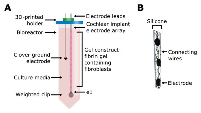
Figure 1 Open in figure viewer PowerPoint Schematic of 3D bioreactor setup. A) Schematic of the tissue-engineered cochlear fibrosis model construct including a cochlear implant electrode array encapsulated with a fibrin gel with 3D-seeded fibroblasts. e1 represents the first/most apical electrode. B) Image of the three apical electrode contacts including connecting wires.

Figure 2 Open in figure viewer PowerPoint Contraction and histology analysis of the constructs. A) Representative image set showing contraction of the construct over the course of the experiment. The length of the construct was calculated using the known mid-to-mid contact spacing of the electrode arrays to calculate the scale of the images for each electrode array and timepoint separately, which was then used to calculate the length of the construct. B) Relative contraction of the constructs, normalized to day 0 absolute length, over time. Single datapoints are shown in grey lines with open circles. Mean ± standard deviation is shown for the stimulated and unstimulated groups (ns = not significant, univariate n-way ANCOVA) in bold as well as all constructs. Relative contraction is significant over time (p < 0.001, univariate n-way ANCOVA) with the inflection point between days 7 and 9 (Tukey's post hoc test). C) Hematoxylin & eosin (H&E) and polarized picrosirius red (PSR) stained histology slices, transverse and longitudinal sections, of two constructs. “*” represents the location of the electrode array. H&E staining shows higher density of cells at the lateral and medial edges of the construct. PSR reveals birefringence and thus collagen formation. No differences between the stimulated and unstimulated constructs are visible.
Next, we performed histology to retrieve information on cellular orientation and extracellular matrix morphology (Figure 2C; Figure S2, Supporting Information). Hematoxylin and Eosin (H&E) staining revealed a higher lateral density of cells with denser medial ECM, indicating cellular repositioning with respect to available nutrients. We performed picrosirius red (PSR) staining for oriented fibrillar collagen[52, 53] to examine for collagen orientation. Some coloration is evident (Figure 2C), indicating that the fibroblasts are producing dense, fiber-like collagen bundles, most likely via mechanical boundary conditions,[54] which are inherently applied by the presence of the CI array. We also utilized a Ki-67 stain, a marker of cell proliferation,[55] to confirm that cells within the constructs where proliferating in all cases (Figure S2, Supporting Information).
Use of electrical stimulation as a method to prevent CI fibrosis has sparked recent interest.[35, 36, 56, 57] Therefore, we tested the effect of stimulation on contraction, while correcting for additional sources of variation. No significant effect of stimulation was found (F = 1.59, p = 0.23, df = 1, univariate n-way ANOVA, relative contraction on day 14-dependent variable, stimulation, electrode design-fixed factors, and experiment number-random factor). We also did not observe any differences from our histological analysis (H&E, PSR, Ki-67). To confirm these similarities, we performed a Hoechst fluorescence assay to quantify DNA at day 14 (Figure S3, Supporting Information). No significant effect of stimulation was found (F = 0.08, p = 0.78, df = 1, univariate n-way ANOVA, DNA per µg dry weight as dependent variable (n = 10), stimulation-fixed factor (n = 4 simulated, n = 6 unstimulated), experiment number-random factor (n = 2 Exp1, n = 4 Exp2, n = 4 Exp3)). These results agree with studies investigating the effects of early switch-on and more extensive stimulation post-operatively, which show little effect on long-term markers of fibrosis formation.[58, 59]
Given that constructs axially contract, we found in some cases, constructs would contract away from electrodes that were covered on day 0. To understand the 3D structure of the constructs relative to positioning along the arrays, samples (n = 2, 1 stimulated, 1 unstimulated) were stained for DNA and actin. The edge and center of the constructs are visible, showing dense cells attached to the arrays (Figure 3A). This allowed us to visualize areas that had become uncovered during contraction, where we observed no evidence of construct remnants. We also observed cellular spreading on an exposed electrode at the trailing edge of the construct (Figure 3B). This observation indicates that cells can adsorb directly onto electrodes, potentially effecting electrode–electrolyte (EE) interface during stimulation. However, as no residual construct remained in areas of arrays that had become uncovered during contraction, this interface is potentially recoverable.


Figure 3 Open in figure viewer PowerPoint Confocal fluorescence imaging of the construct. 3D orientation of the construct, as fixed on day 14, related to the electrode array. The nuclei are stained blue via DNA staining with Hoechst 33258, while actin was stained with phalloidin-iFluor 594 showing in red. A) Edge and mid-construct images without stimulation. B) Total and close-up of a stimulated construct. Both constructs show attachment of the cells on the electrode surfaces. Actin fibers in the cells can be seen spreading out over the surface of the electrodes and numerous cells are attached to a singular electrode alone.
Within the statistical tests described in this section, an effect of experiment number was found on relative contraction and DNA quantification (Figures S1C and S3, Supporting Information), possibly indicating some variance within the fibroblast cell line used for this study.
2.2 Electrochemical Impedance Spectroscopy Shows Significant Changes in the Bulk of the Gel
We hypothesized that complex impedance would change as measured via EIS with cellular contraction and construct remodeling. To test this hypothesis, we tracked complex impedance spectra over six timepoints to day 14. These spectra were fitted to a circuit model (Figure 4A), consisting of a constant phase element (CPE) representing EE interface, a resistor (R1) in parallel with a capacitor (C) representing the bulk of the construct, and an additional resistor (R2) representing the resistance of the media and ground. Since we did not expect a major contribution to overall impedance with changes in cell media and pathway to ground, R2 was fixed based on the earliest available timepoint for each electrode. The EE interface and bulk of the construct have been hypothesized to change during cochlear fibrosis.[35, 36, 39, 60, 61] So, these elements were fitted without constraints. The average weighted sum-of-squares, proportional to the average percentage error between original and fitted data, was <1% for most fittings and at least <5% for all fittings (Figure S4A, Supporting Information). An example of impedance magnitude and phase angle over time, for both measured and modeled data, for 1 electrode with the construct on throughout the experiment can be seen in Figure 4B and without construct in Figure S4B (Supporting Information). An increase in absolute impedance magnitude is seen at higher frequencies (>10 kHz), while phase angle decreased across most frequencies in this example.

Figure 4 Open in figure viewer PowerPoint Complex impedance measured with electrochemical impedance spectroscopy (EIS). EIS was measured on all electrodes, regardless of having an open circuit (e.g., air bubble or broken electrode). The exclusion criteria, as described in the materials & methods section, led to n = 231 recordings with construct and n = 153 without construct being included (of a combined total of n = 528 recordings). A) Proposed equivalent circuit of the 3D bioreactor model with a constant phase element (CPE) representing the electrode-electrolyte (EE) interface, a resistor (R1) in parallel with a capacitor (C) representing the bulk of the construct, and an additional resistor (R2) representing the media and ground (GND). B) Absolute impedance magnitude and phase angle of an example electrode over time, showing both measured and modeled values. Measured data are shown as mean ± standard deviation. C) Modeled circuit elements over time of all timepoints and electrodes with construct (and thus modeling fibrosis) on the electrode. Individual data are shown in grey. The arithmetic mean ± standard deviation is shown in bold black, except for C where the geometric mean and standard deviation is shown. CPE-P and CPE-T show no significant (ns) changes from day 2 to day 14 (univariate n-way ANOVA, Tukey's post hoc test). R1 shows a significant increase from day 2 to day 14 (****p < 0.001, univariate n-way ANOVA, Tukey's post hoc test), while C shows a significant decrease (****p < 0.001, univariate n-way ANOVA, Tukey's post hoc test).
Fitted circuit elements over time with construct on showed CPE phase (CPE-P) and magnitude (CPE-T) stay constant, while circuit element R1 increased and C decreased (Figure 4C). This change is not seen for electrodes without constructs on them (Figure S4C). R1 showed a large significant effect of time (F = 21.51, p < 0.001, df = 5), with the inflection point between days 7 and 9 as revealed by Tukey's post hoc test, and overall significant change between day 2 and day 14 (p<0.001). C also showed a large significant effect of time (F = 15.12, p < 0.001, df = 5), with the inflection point between days 4 and 7 as revealed by Tukey's post hoc test, and an overall significant decrease between days 2 and 14 (p < 0.001). CPE-P and CPE-T remained largely. When comparing to fitted circuit elements for electrodes without construct, no significant effect of time is found for CPE-P (F = 1.06, p = 0.38, df = 5), CPE-T (F = 0.79, p = 0.56, df = 5), R1 (F = 0.78, p = 0.56, df = 5), and C (F = 1.85, p = 0.11, df = 5). Overall, these data suggest changes in EIS can be explained by an increase in resistance and decrease in capacitance of the bulk of the construct with no significant changes in EE interface seen.
A commonly studied circuit to model contact impedances in relation to cochlear fibrosis was introduced by Tykocinski et al. and includes a resistor in parallel with a capacitor representing EE interface and a single resistor in series representing the bulk of tissue (Figure S5A, Supporting Information).[62] This circuit is extracted from a voltage waveform (contact impedance timepoints) and models access resistance, initial increase in voltage at the start of the waveform, and polarization impedance, the capacitive build-up after access resistance.[62] Changes in polarization impedance have since been linked to protein adsorption (increase) and resorption (decrease) on the electrode.[35, 39, 57] Changes in access resistance are more commonly associated with changes in bulk tissue surrounding the electrode, where an increase in access resistance is linked to an increase in tissue formation.[36, 39, 56, 60] However, changes are not specific to new tissue formation only, as an increase in access resistance has also been associated with electrode-modiolus distance, translocation of the electrode from one scala to another intracochlearly, extracochlear electrodes, and electrode failure.[63-67] We fitted this circuit to our example data (Figure 4B; Figure S5B, Supporting Information) mainly showing a large error in phase angle for complex impedance. Average weighted sum-of-squares was >10% in all six timepoints (Figure S5C, Supporting Information), suggesting this circuit is too simple to model complex impedance for our model of fibrosis.
2.3 Contact Impedances and Second Phase Peak Ration (SPPR) of Voltage Waveforms Increase Significantly Over Time
To translate the changes in complex impedance to an electrical measurable in patients, we measured voltage waveforms at all timepoints for electrodes with and without construct on (Figure 5A; Figure S6A, Supporting Information). Generally, an increase in voltage over time is observed with construct on the electrode, while no changes are seen without construct on the electrode. When the construct contracts off an electrode, the voltage waveform was seen to normalize back to the level of the waveform at day 2 (Figure S6B).
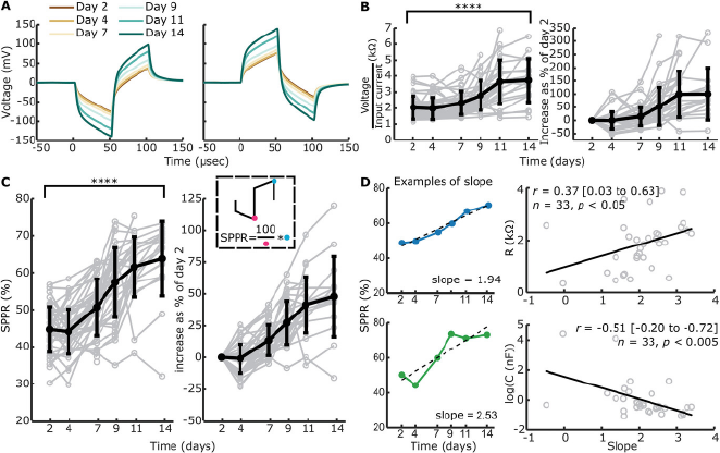
Figure 5 Open in figure viewer PowerPoint Measured voltage waveforms, contact “impedances” and SPPR over time. Voltage waveforms were only measured when EIS measurements were included and a single pulse did not elicit high voltage waveform responses, leading to n = 221 with construct and n = 115 without construct. A) Example mean voltage waveforms over time for the same electrode as in Figure 4B, with a cathodic-leading biphasic pulse and anodic-leading biphasic pulse as an input. B) Absolute and relative contact “impedances” over time. Individual traces are shown in grey, while mean ± standard deviation is shown in bold black. Absolute contact “impedances” significantly increased over time from day 2 to day 14 (****p < 0.001, univariate n-way ANOVA, Tukey's post hoc test). C) Absolute and relative SPPR shown over time. Individual traces are shown in grey, while the mean ± standard deviation is shown in bold black. A schematic of how the SPPR is calculated is shown (second phase peak as a percentage of the first phase peak). Absolute SPPR significantly increased over time from day 2 to day 14 (****p < 0.001, univariate n-way ANOVA, Tukey's post hoc test). (D) Example of linear function fitting to SPPR over time including the output slope are shown for a relatively good (blue) and bad (green) fit. The linear function is shown as a dashed black line. The slope of the linear fit is significantly positively correlated with R1 as fitted with EIS and significantly negatively correlated with C as fitted with EIS (Pearson's correlation coefficient).
Contact impedances, voltage at the end of the first phase of a cathodic-leading pulse normalized to the input current, were calculated with (Figure 5B) and without (Figure S6C, Supporting Information) constructs on the electrode. Contact impedances with construct on the electrode were normalized to day 2. Contact impedances significantly increased over time when construct was on the electrode (F = 23.91, p < 0.001, df = 5, univariate n-way ANOVA corrected for experiment number (random factor)), with inflection point between days 7 and 9 as revealed by Tukey's post hoc test, and an overall significant change between days 2 and 14 (p < 0.001). Without construct on the electrode, no significant changes were seen over time (F = 1.32, p = 0.26, df = 5).
We hypothesized that with an increase in R1 and a decrease in C over time for electrodes with construct on, ratio of the second peak as a percentage of the first peak would change over time, as the contribution of capacitive discharge to the second phase peak would decrease. Therefore, we calculated the second phase peak ratio (SPPR) as shown in Figure 5C, which describes second peak voltage as a percentage of the first peak voltage. The SPPR increased significantly over time when the construct was on the electrode (F = 38.05, p < 0.001, df = 5, univariate n-way ANOVA corrected for experiment number (random factor)), with the inflection point between days 4 and 7 (Tukey's post hoc test). Here, a significant difference was found between days 2 and 14 (p < 0.001). Without construct on the electrode (Figure S6D, Supporting Information), no significant changes were seen with time (F = 1.07, p = 0.38, df = 5).
To compare change in SPPR over time with a single measure to EIS-fitted circuit elements R1 and C, we calculated slope of SPPR over time with a linear function. Two examples of such slopes can be seen in Figure 5D, with both SPPR that shows a linear increase over time and one that does not. We only fitted data to a linear function when >3 datapoints and datapoints after day 7 (inflection point of R1) were available, leading to n = 33 slopes. These slopes were correlated with the final available timepoint used for the linear fit (Figure 5D) of EIS-fitted circuit elements. A significant positive correlation was found between the SPPR and R1 (Pearson's r = 0.37 (95% CI: 0.03 to 0.63), p < 0.05, n = 33), while a significant negative correlation was found between SPPR and C (Pearson's r = −0.51 (95% CI: −0.20 to −0.72), p < 0.005, n = 33).
2.4 Voltage Waveform-Fitted Circuit Elements Correlate Significantly with EIS-Fitted Circuit Elements
To expand information extraction from voltage waveforms, we reverse fitted (voltage waveform (VW) fitted) (Figure S7A, Supporting Information) our chosen circuit (Figure 4A) to the voltage waveforms (Figure 6A). R1 and C show similar trends, yet capacitance is higher for the VW-fitted example. Additionally, C is capped at its upper limit (102 nF) for days 2 through 7.
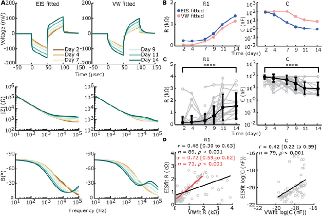
Figure 6 Open in figure viewer PowerPoint Reverse fitting of voltage waveforms (VW) to electrical circuit. A) EIS-fitted and VW-fitted voltage waveforms (top row), absolute impedance magnitude (middle row), and phase angle (bottom row) of electrical circuit in Figure 4A on example data shown in Figures 4B and 5A. B) Example of direct comparison between EIS-fitted (blue) and VW-fitted (pink) circuit element sizes for the example shown in (A). C) VW-fitted circuit elements over time of all timepoints and electrodes with construct on the electrode (n = 193). Individual data is shown in grey. The arithmetic mean ± standard deviation is shown in bold black, except for C where the geometric mean and standard deviation are shown. R1 shows a significant increase from day 2 to day 14 (****p < 0.001, univariate n-way ANOVA, Tukey's post hoc test), while C shows a significant decrease (****p < 0.001, univariate n-way ANOVA, Tukey's post hoc test). D) Correlation between VW-fitted and EIS-fitted R1 and C, excluding uncapped values (including n = 89 for R1 and n = 79 for C, compared to n = 193 for both) as part of the bimodal distribution seen in Figure S7C (Supporting Information). A significant but modest correlation was found for both circuit elements (Pearson's correlation coefficient). For R1, the correlation is stronger when VW-fitted elements >2 kΩ are excluded, suggesting outliers are more likely with R1 > 2 kΩ in VW-fitting.
CPE-P and CPE-T were fixed based on day 2 values in addition to fixed R2 values, and so only data with EIS fitting available on day 2 was included (Figure 6C). R1 increased significantly over time (F = 17.83, p < 0.001, df = 5, univariate n-way ANOVA corrected for experiment number (random factor)), whilst C decreased significantly over time (F = 23.98, p < 0.001, df = 5). The inflection point, as shown by Tukey's post hoc test, was in between days 7 and 9 for R1 and days 4 and 7 for C. Significant differences from days 2 to 14 were present for both R1 (p < 0.001) and C (p < 0.001).
A percentage of VW-fit output shows capped values where R1 caps its lowest bound of 50 Ω and C caps its upper bound of 10−7 F. Capping mainly happens when the voltage waveform peak is at its lowest, since 60.6% of the output values is capped in at least one element over all timepoints, whilst from days 9 to 14, only 21% of the VW-fittings is capped (Figure S7B, Supporting Information). This leads to a bimodal distribution for output values of VW-fitted R1 and C with the element bounds used (Figure S7C, Supporting Information). Widening the element bounds, however, leads to capping at both bounds for both circuit elements (Figure S7D, Supporting Information). To compare EIS-fitting with VW-fitting we correlated EIS-fitted values of circuit elements R1 and C to VW-fitted values of the same electrode and timepoint. A significant positive correlation was found between EIS-fitted R1 and VW-fitted R1 (Pearson's r = 0.48 (95% CI: 0.30 to 0.63), p < 0.001, n = 89). However, outliers were seen when VW-fitted R1 reached >2 kΩ. Excluding VW-fitted R1 > 2kΩ showed a stronger correlation between VW-fitted and EIS-fitted R1 (Pearson's r = 0.72 (95% CI: 0.59 to 0.82), p < 0.001, n = 73). A significant positive correlation was also found between EIS-fitted C and VW-fitted C (Pearson's r = 0.42 (95% CI: 0.22 to 0.59), p < 0.001, n = 79).
2.5 Changes in Contact Impedances and SPPR in CI Patients Postoperatively are in Line with Changes Found in the Tissue Engineered Model
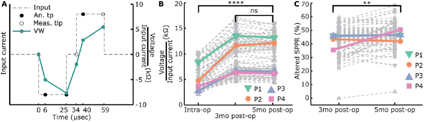
Based on our findings of SPPR changes in our tissue-engineered model, we wanted to test this marker in recently implanted CI patients. We used the CI company's software function to measure mutliple timepoints along voltage waveform response, to measure an altered version of SPPR (6 µs into each phase) as well as compare this to the contact impedances (Figure 7A) over 2 and 3 timepoints, respectively, in four patients. We assumed no or little fibrosis was present before cochlear implantation, since these were new CI patients, and at least some fibrosis formation to occur within 5 months postoperatively. It should be noted that, given the inability of currently-used diagnostics to monitor fibrosis progression, we have no independent information about fibrosis status at the collected timepoints.